The ability to import font types into Hyperion Financial Reporting is a common request by many companies, typically a request resulting from corporate reporting standards. Not only is this possible, it’s a quick and easy exercise that is detailed out below.

Step 1: Locate the Font Folder.

The font type files (normally identified by a .TTF or .ttf extension) can be found in the “Fonts” folder located in your Windows directory (Likely on your ‘C’ drive). The key here is locating this folder on the server where Hyperion Financial Reporting has been installed.

Step 2: Copying& Pasting the New Font File.

This is as easy as it sounds… just copy and paste the new file into this directory.

Step 3: Creating a Report.

Opening Hyperion Financial Reporting and create/modify a report. When selecting the font type, notice the new Font Type that was just added in Step 2 above. Note that it’s best to close the Financial Reporting client before importing the new Font file onto the server; this will insure that the client will recognize the new file.


Reporting solutions often require companies to filter out a top range of Key Performance Indicators; for example, the top 10 expenses related to marketing. Hyperion Financial Reporting makes this type of reporting easy for developers by providing the “Top” properties checkbox. The difficulty arises when a company requires a solution to display the bottom 10 – those 10 expenses that account for a majority of marketing related expense. Hyperion Financial Reporting has nothing built to provide this type of information.

As you might expect – knowing your smaller expenses is important but knowing the largest; those where you can improve margin, is vital. A solution to display the bottom 10 is detailed below; this solution displays the 10 largest negative values vs. displaying the 10 largest positive values.

The high-level solution includes the following functionality:
a.    Inserting a “Rank” column.
b.    Sorting on the “Rank” column.
c.    Adding conditional suppression for bottom 10.

Step 1:

Create a report grid with a formula column as the first column (Column A below).


Step 2:

Insert the “Rank” function on the Formula Column. Be sure to choose the “Ascending” property. Adding “Rank” will order the rows from High-to-Low based on the data returned. The example below provides ranking off of Column ‘A’. The ranking is used on Step 4 when adding conditional suppression.

Step 3:

Apply row “Sort” to the grid. You find the “Sort” property by placing focus on the entire grid (left clicking the upper left-most cell). Choose to apply sorting to the “Rows”, Sort by “Column A”, and sort in “Ascending” order. Sorting will determine the order in which the data is displayed, Ascending or Descending. The Sorting is used on Step 4 when adding conditional suppression.

Step 4:

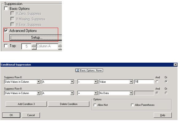
Add Conditional Suppression to the row(s). This logic will determine which data rows are ultimately displayed to the user. To add conditional suppression, highlight the row and click “Advanced Options”. Because the requirement is to show the bottom 10, suppression should hide any row with a “Rank” value greater than 10 (You will also want to suppress rows where “No Data” is returned).

When this report is run, only the bottom 10 will be displayed to the user… those marketing expenses with the largest negative values. The solution above will essentially do what a “Bottom” checkbox would have provided had Hyperion programmed this functionality into the application.


When I am introduced to business segments that use Hyperion Essbase, I always get asked the same question: “Can you explain what sparse and dense mean?”  Although I agree that users don’t HAVE to understand the concept, I contend that it is extremely valuable if they do.  It will not only help them become more efficient users, it goes a long way in helping them understand why something simple in Excel isn’t always simple in Essbase.  If users understand what a block is, and what it represents, they have a much better experience with Essbase.

If you are a relational database developer or a spreadsheet user, you tend to view data in 2 dimensions.  An X and Y axis is equivalent to the rows and columns in your spreadsheet or database table.  Essbase is a little different in that it stores data in 3 dimensions, like a Rubik’s Cube, so it has a Z axis.  Essbase databases refer to these “Rubik’s Cubes” as blocks.  An Essbase database isn’t one giant Rubik’s Cube; it could be millions of them.  The size and number of possible blocks a database has is determined by the sparse/dense configuration of the database.

An Essbase outline has a number of dimensions.  The number of dimensions can range in quantity and size, but each dimension is identified as a dense or sparse dimension.  The dense dimensions define how large each block will be in size (the number of rows, columns and the depth of the Z axis).  The sparse dimensions define the number of possible blocks the database may hold.  Assume the following scenario:  a database exists with 3 dense dimensions and 2 sparse dimensions.  The dense dimensions are as follows:

Net Income
Income
Expenses

Qtr 1
Jan
Feb
Mar

Version
~ Actual
~ Budget
~ Forecast

Remember, the dense dimensions define the size of blocks.  These dimensions would produce a block that looks like the image below.  Every block in the database would be the same.

For those more knowledgeable with Essbase design, this example assumes that no member is dynamically calculated or is tagged as a label to reduce complexity.


The sparse dimensions are below.

Total Product
Shirts
Pants

Total Region
North
South
East
West

The unique combinations of each sparse dimension has its own block.  There will be a block for Pants – North, one for Shirts – North, and so on.  Since there are 3 members in the Total Products dimension and 5 members in the Total Region dimension, there will be a total of 15 (3 x 5) blocks.  If a database has 5 sparse dimensions, all with 10 members, it would have a total possible number of blocks equal to 100,000 (10 x 10 x 10 x 10 x 10).  Below is a representation of the possible blocks for Shirts.


Many developers that work with Hyperion products, as well as many any other software product, use virtual machines.  Virtual machines are an easy way to create multiple environments for testing and developing multiple product versions

The 3 main applications to create and use virtual machines are

I have used all 3.  Opinions can be found that promote all 3.  Many IT professionals prefer VMWare.  I have found it to be a little cumbersome to use, and find sharing virtual machines to be a frustrating experience.  I am not a stereotypical IT professional, but rather a business person with an aptitide for technology.  That said, I prefer VirtualBox.  For me, VirtualBox is easier to install and manage the virtual machines.  It is easy to move virtual hard drives to another computer, simple to duplicate a virtual hard drive and allows users to take snapshots, which allows, for lack of a better explanation, a huge undo if required.

Through my VirtualBox travels, I have found the following knowledge to be very valuable.  Here are some HOW TOs that might be useful if you decide to use Sun’s VirtualBox.

How to reduce the size of a virtual machine
The use of virtual machines (just like any system) cause fragmentation and the size of the virtual hard drive to grow, sometimes substantially.  Managing the size of the virtual machine is relatively easy, and is not time consuming.  It involves 3 actions (defrag, delete free space, and compact the virtual hard drive).  Here is one way to accomplish reducing the size of your virtual machine / virtual hard drive.

  1. Open the virtual machine that needs compressed
  2. Download sDelete, and extract the sDelete.exe to c:\
  3. NOT REQUIRED:  Download and install Smart Defrag – this is a free disk defrag tool that I have found to be more effective than the one that comes with the Windows OS.
  4. Use the disk defrag tool that comes with Windows or the one above, and defragment the hard drive.
  5. Go to Start/Run, and enter “c:\sdelete.exe -c”
  6. Shut Down the OS on the virtual machine
  7. On the host computer, open a command window (Start/Run, and enter cmd)
  8. If VirtualBox was installed in the default location, change the directory to the VirtualBox directory by entering “cd C:\Program Files\Sun\xVM VirtualBox\”
  9. Enter “VBoxManage modifyvdi HardDrivePathAndName compact” where HardDrivePathAndName is the full path to the hard drive the virtual machine is using.

If the virtual machine/hard drive has free space, this process will find it and reduce the overall size of your virtual machine/hard drive.

How to duplicating, or clone, a hard drive
Often times there is a need to replicate a virtual machine on the same host environment.  Copying the file doesn’t do the trick, as every virtual machine’s hard disk must have a unique key.  VirtualBox comes with a tool to duplicate the hard drive and assign it a new key.  To accompolish, follow the following steps.

  1. Reduce the hard drive size (see previous topic)
  2. On the host computer, open a command window (Start/Run, and enter cmd)
  3. If VirtualBox was installed in the default location, change the directory to the VirtualBox directory by entering “cd C:\Program Files\Sun\xVM VirtualBox\”
  4. Enter “VBoxManage clonevdi Source Destination” where Source is the full path to the hard drive the virtual machine to duplicate and Destination is the location of the new virtual machine hard drive.
  5. Open VirtualBox and create a new virtual machine that points to the newly created hard drive in the previous step.


Comparing the current period to the prior period is relatively easy to accomplish in Essbase, and is often required when creating a Cash Flow hierarchy.  Assume the following scenario.

An outline exists that includes a Year and Time_Period dimension. The Year dimension includes 2007, 2008, and 2009.  The Time_Period dimension includes Full Year, Quarter 1 through 4, and all 12 months.  The dimension type for the Time_Period dimension has to be set to Time.  A dimension named COA (chart of accounts) holds the general ledger account structure. Below is an example of the Time_Period dimension

To enable a dynamic approach to solving this problem and minimizing the maintenance required as new years are added, an understanding of the following two functions is required.

@PRIOR
The PRIOR function provides a way to compare a member outside of the Time_Period dimension in multiple Time_Period members.  For example, accounts for July could be compared to June, or Quarter 2 could be compared to Quarter 1.  There are two parameters that this function accepts.  The first is the member to get the prior value for.  The second is the number of periods you want to shift the comparison.  If @PRIOR(“Asset123”,1) is used, it would provide the value for the period previous to what you had selected in the Time_Period member.  So, if June was selected, it would provide the value for May. If the formula was @PRIOR(“Asset123”,2) and June was selected, the result would be the value for April (2 periods back).  The function uses members at the same generation, so @PRIOR(“Asset123”,1) would provide the difference between Qtr2 and Qtr1 if Qtr2 was selected.

So, what happens if January or Qtr1 is selected?  There is no previous member for these.  This is where the second function comes in to play.

@MDSHIFT
MDSHIFT is similar to PRIOR, but it lets the calculation reference members across dimensions.  Where PRIOR only allows references on one dimension, MDSHIFT allows references to move across multiple dimensions.  If the user expects to see the different between Jan and Dec of the prior year or Qtr1 to Qtr4 of the prior year, MDSHIFT enables that to happen without hard coding the script.  Again, the goal is to have a script that doesn’t need to be maintained.

MDSHIFT accepts a set of parameters.  If your shift needs to occur along one dimension, it requires one set of parameters.  If your shift needs to occur along more than one dimension, it will accept multiple sets.  The function’s first parameter is the member you are evaluating, just like the PRIOR function.  The next set of parameters is what can exist multiple times if you are shifting along multiple dimensions.  The set consists of three parameters, of which the first two are required.  The first of the set is the number of positions to shift.  The second is the dimension to shift on.  The third is a range of member to use to shift along.  If this is left blank, Essbase uses level 0 members.

To get the prior value for Jan, or Dec of the previous year, it would be MDSHIFT(“Asset123″,-1,”Year”,,11,”Time_Period”,).  The first parameter is the member to evaluate.  The next two parameters are used to reference the previous member (-1) in the Year dimension.  Since the Year dimension members are level 0, the fourth parameter is not required.  The next series, or set, references Dec ( 11, or move forward 11 from Jan) of the Time_Period dimension.  The last parameter is not required since we only want to reference level 0 members again.

Putting it all together
If we put these two functions together with a basic if/then/else statement, we get a dynamic formula that won’t need to be updated as we progress through time.  It would look something like this:

If(@ISMBR(“Jan”))
  /* if Jan, then we have to compare Jan in the current year to Dec [shift 11] in the prior year
[shift -1]  */

“Asset123” – @MDSHIFT(“Asset123″,-1,”Year”,,11,”Time_Period”,);
ELSEIF(@ISMBR(“Qtr1”))
/* if Qtr1, then we have to compare Qtr1 in the current year to Qtr4 [shift 3] in the prior year
[shift -1]
The last parameter includes a range since we are not using level 0, which is the default  */

” Asset123″ – @MDSHIFT(“Asset123″,-1,”Year”,,3,”Time_Period”,(“Qtr1″,”Qtr2″,”Qtr3″,”Qtr4”));
ELSEIF(@ISMBR(“YearTotal”))
/* if Year, then we have to compare to last year [shift -1] */
” Asset123″ – @MDSHIFT(“Asset123″,-1,”Year”,);
ELSE
    /* all other members, which would include Feb through Dec */
” Asset123″ – @PRIOR(“Asset123”,1);
ENDIF;

 
Executing calculations that only run on blocks that have changed is a great feature in Essbase.  It enables administrators to calculate the database in a fraction of the time and is referred to as calculating “dirty” blocks, or an update calc.  This is awesome.  “Why shouldn’t I use it all the time?” you might ask.  Understanding how the Essbase calc engine works is critical to answering this question.

The Essbase calc engine calculates each block in a specific order (see figure 1).  The first block it calculates is the first level 0 block of the first sparse dimension.  It then traverses to higher levels and moves through the dimension from top to bottom until the entire dimension is consolidated.

When a level 0 block is changed, it and all of its parents, are tagged as dirty (it needs to be calculated again). When a calculation is executed on just dirty blocks, the process is the same except that it skips all the “clean” blocks.  Once the block is calculated the dirty tag is changed to clean.  So far, so good!

Revisit figure 1, which is a very simple example.  It shows a very simple hierarchy with the order in which the blocks are calculated, 1 through 10.

Figure 2 shows what happens if New York is updated.  Blocks 5, 6, and 10 are tagged as dirty.  The next calculation, if set to calculate only the dirty blocks, would only calculate blocks 5, 6, and 10, in that order.

Here is where things get a little ugly.  When an application has write access, as a planning or forecasting application would, it is very possible that users are updating data DURING the calculation process.  The timing of these events is critical to understand why calculating only dirty blocks can cause inconsistencies.

When a calculation has started, it identifies which blocks need calculated (5, 6, and 10 in this example).  Immediately after that, it starts calculating block 5.  If Texas is updated while block 5 is being calculated, what happens?

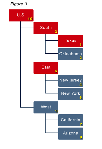
Figure 3 shows the state of the clean/dirty blocks when the calculation is finished with block 5.  It is exactly what you might expect at this point.  Blocks 6 and 10 are still dirty.  The update of Texas caused Blocks 1, 3, and 10 to be tagged dirty.

This is the critical piece.  Keep in mind how the calculation engine works.  It will continue to calculate blocks 6 and 10.  Also note that the calculation running does NOT reevaluate what needs calculated.  It will not calculate blocks 1 and 3.

Figure 4 shows the state of the blocks after the calculation finishes.  Only blocks 1 and 3 are dirty at this point because 10 was included in the calculation.

When the next calculation is executed, the only blocks that are dirty are 1 and 3.  Can you see the problem now?  After blocks 1 and 3 are calculated, is block 10 accurate?  Does U.S. equal the total of South, East, and West?  Unfortunately, it does not.

One could argue that it will get updated the next time data is changed.  In a very simple example with 3 levels, this would probably correct itself rather quickly, if the problem happened at all.  In a more realistic example where a company has 10 or 20 levels in their organization dimension, the problem is likely to be a reoccurring problem and may not be corrected until a full calculation is executed.  In most situations, it is not acceptable to have a database where it consolidates correctly only some of the time without any warning that it is not accurate.  Reporting can be incorrect, and bad management decisions can result.

Using the dirty calc feature is a great tool to have in your arsenal.  It can save hours of processing time.  It can make you look like a genius.  Without understanding its pitfalls, it can be the source of countless wasted hours trying to figure out why a cube isn’t consolidating correctly.  A worst case scenario is when a cost center manager updated their budget, it never gets consolidated correctly, and the problem isn’t identified until it is too late.


Overview

Essbase is widely considered to be the industry leading OLAP (On-Line Analytical Processing) server. Built on a real-time analytic infrastructure, Essbase provides BI and EPM users the ability to quickly dissect and analyze data through an intuitive interface.  Essbase end-users have multiple options for interacting with data including Microsoft Excel, Hyperion Financial Reporting and Hyperion Web Analysis. By bringing Essbase together with other Oracle applications, users will find broad support for demanding business requirements.  Breaking down large datasets, working with best-case/worst-case scenarios, forecasting multi-line expenses, and reporting variance analysis is now at your fingertips. Essbase ultimately allows end-users to interact and analyze real-time data through an integrated, rapid-response, and secure environment.

Product History

Arbor Software Corporation, an OLAP software company that designed and marketed multidimensional database software for planning and analysis, developed Essbase (Extended Spreadsheet Database), first branded “Arbor Essbase” in 1992. This multidimensional database product was originally developed to address the scalability problems associated with spreadsheets like Microsoft Excel and Lotus 1-2-3.

In 1998, Hyperion Software Corporation, a company with packaged analytic applications specializing in financials, and Arbor, merged to become Hyperion Solutions Corporation. Their first assignment after the merger was obvious, integrating Essbase with Hyperion Pillar, Hyperion Enterprise, and Hyperion Reporting.

After the merger, Essbase became the backbone to a full suite of applications for planning & budgeting, financial consolidations, scorecards, reporting, and more. Hyperion Solutions become a leader in the world of performance management software with Essbase leading the way.

In 2007, Oracle purchased Hyperion Solutions. At the time of the acquisition, Hyperion applications were being used by approximately 12,000 companies, including 91 of the Fortune 100. The acquisition made Oracle a leader in the EPM (Enterprise Performance Management) market and strengthened the Oracle offerings.

Strengths / Benefits


In2Hyperion is a consortium of experts in a field often referred to as Business Intelligence, Enterprise Performance Management, and a host of other fancy acronyms. The focus of this effort will be around the Oracle Hyperion suite of products, but won’t be limited to them.

This space has been developed to help inspire people to search and implement betters ways of doing the same old thing.  Whether it be using a more appropriate software solution, or using your existing assets in a more efficient and effective way, we believe there is a lot that can be done to overcome our current challenges.  We intend to grow this website to create a rich resource that those inside and outside of this industry can tap in to and become more effective.  Inspire us by posting comments and sharing your experiences so we can grow as a team, and help more and more of our friends in the BI spectrum.