Convert a Planning Load File to an Essbase Load File

There are a ton of reasons to convert a planning load file to an Essbase load file.  Maybe you are migrating a file from one environment to another, or simple want to load the file faster, but there are reasons to use the Essbase format.

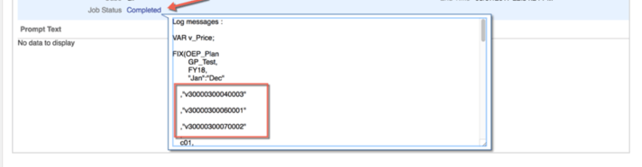
Oracle is working on an enhancement that should be released in the next month or two that will use a load rule to load data to the app using the Essbase load format, which means the logging will be much improved, it won’t stop at the first failed line, and it will log all the errors, just like the Planning load format.  That is great news for those of us that use the planning format purely for the logging.

Performance

Before I get into the script, I want to touch on the speed of this method.  The file I used, based on a real situation, was over 89 million lines (yes, that is correct, million), and took over 5 hours to load as a Planning file.  It had to be split into three files to be under the 2GB limit, but it successfully loaded.  The file was received late in the morning and had to be loaded before the start of the day, so a 5 to 6-hour processing time was unacceptable.  By the way, yes, the file was sorted appropriately based on the sparse and dense settings.

I was able to build a unix/linux script using awk to convert this file to an Essbase load format and it only took about 9 minutes to convert.  The improved load time was pretty drastic.  It finished in under 15 minutes.

For testing, it was great, and it was perfect to improve the processing until the source system could rebuild the export in the Essbase format.  Just to reiterate, I added less than 10 minutes to convert the file, and reduced the load time by 4.5 hours, so it was worth the effort.

The Catch

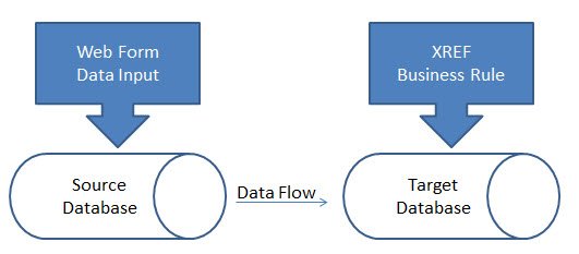
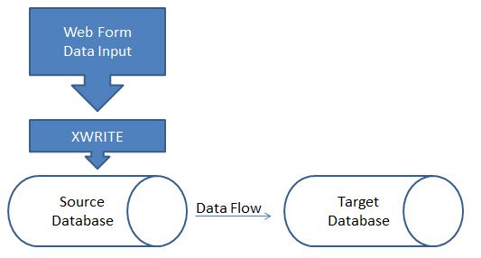
Before I continue, if you are unfamiliar as to why the two load formats, here is the difference.  Essbase loads the data directly to Essbase.  The Planning load will bounce the file off the Planning repository to convert any smart list string account to the appropriate number, which is what is stored in Essbase.  This process creates a new file on the server, in an Essbase load format, with the numeric representation of each smart list account.  If you have no smart list conversions, this entire process is done for no reason, which was the case in this situation.  So, this isn’t the answer in every situation.

The Script

Before I get into the script, if you know me you know I love my Mac.  One of the reasons is because I have the performance of a Mac, I can obviously can run Windows whenever I want, and I have the ability to run Bash scripts through the terminal.  I am not a Bash scripting expert, but it is extremely powerful for things like this, and I am learning more as I need to build out functionality.

If you are a Windows user, you can install and use Linux Bash scripting in Windows 10.  You can read about it here.

There are several languages that can be used, but I chose AWK, which is a domain-specific language designed for text processing and typically used as a data extraction and reporting tool. It is a standard feature of most Unix-like operating systems.

First the script.  Here is it.  I put the awk on multiple lines so it was a little more readable, but this is one command.

SOURCEFILE="Data.csv";
LOADFILE="DataLoad.csv";
HEADERMBR=$(head -1 $FILE | cut -d ',' -f2)

awk -v var="$HEADERMBR" 
     'BEGIN {FS=","; OFS="\t"} 
     NR>1 
     {gsub(/"/, ""); 
          print "\""$1"\"", "\""$3"\"", "\""$4"\"", 
                "\""$5"\"", "\""$6"\"", "\""$7"\"", 
                "\""$8"\"", "\""var"\"", $2}' 
     $SOURCEFILE > $LOADFILE;

There are a few things you will need to change to get this to work.  Update the source file and the load file to reflect the file to be converted, and the file name of the converted file, respectfully.  Inside the AWK script, I have 8 fields, 1 through 8.  This represents the 8 columns in my Planning file, or the dimensions and the data.  Your file might have a different count of dimensions.  If your file has more or less delimited columns (ignore the POV field quotes and assume that each delimited field in that is an additional field), update the script as needed

In this example is a planning file example and each arrow represents a field.  The print section of the awk command changes the column order to fit what the Essbase load format requires.

Breaking down AWK

This won’t teach you everything there is to know about AWK, as I am still learning it, but it will explain the pieces used in this command so you can get started.

This piece is simply creating two variables, the source file and the converted file name, so there aren’t multiple places to make these changes when the script needs updated.

SOURCEFILE="Data.csv";
LOADFILE="DataLoad.csv";

The head command in Linux grabs specific lines, and -1 grabs the first line of the file.  I pipe that with the cut command to grab the second field of the header line, which is the dimension member I need to add to every row.  That gets stored in the HEADERMBR variable for later use.

HEADERMBR=$( head -1 $FILE | cut -d ',' -f2)

The example file above is repeated here.  You can see that the second field is the member and HEADERMBR is set to source_SAP.

Now the AWK command.  Before I jump into it, the AWK looks like this.

awk 'script' filenames

And in the script above, the awk script has the following form.

/pattern/ { actions }

You can also think of pattern as special patterns BEGIN and END.  Therefore, we can write an awk command like the following template.

awk '
     BEGIN { actions }
     /pattern/ { actions }
     /pattern/ { actions }
     ……….
     END { actions }
' filenames

There are also a number of parameters that can be set.

This script starts with a variable.  The -v allows me to create a variable.  The first part of this command creates a variable named var and set it equal to the HEADERMBR value.  I have to do this to use the variable in the script section.

-v var="$HEADERMBR"

The BEGIN identifies the delimiter as a comma and sets the output delimiter to a tab.  FS and OFS are short for Field Separator and Outbound Field Separator.

'BEGIN {FS=","; OFS="\t"}

Since the file has a header file, and I don’t want that in my Essbase load file, I only include the lines greater than 1, or skip the first line.  NR>1 accomplishes that.

NR>1

Gsub allows me the ability to create substitutions.  The source file has quotes around the POV field.  AWK ignores the quotes, so it interprets the field with the start quote and the field with the end quote as a field with a quote in it.  These need to be removed, so the gsub replaces a quote with a blank.  The first parameter is a literal quote so it has to be “escaped” with a /.

gsub(/"/, "");

The next piece is rearranging the columns.  I want to have the second column, or the column with the data, at the end.  I have 8 columns, so I put then in the order of 1, skip 2, 3 through 8, then the variable that was created that has the dimension member in the header line, then 2(the data field).  It looks a little clumsy because I append a quote before and after each field, which is required for the Essbase load format.  But, this is just printing out the fields surrounded by quotes (except for field 2, the data field) and separated by columns.

print "\""$1"\"", "\""$3"\"", "\""$4"\"", "\""$5"\"", "\""$6"\"", "\""$7"\"", "\""$8"\"", "\""var"\"", $2

The last piece is identifying the file I want to do all this work to.

$SOURCEFILE

I want to send the results to a file, not the screen, and the > tells the command to send the results to a new file.

> $LOADFILE

The Result

The outcome is a file that is slightly larger due to the additional quotes and replicating the member from the header in every row, normalizing the file.  It is converted to a tab delimited file rather than a comma delimited file.  The header is removed.  The app name is removed.  And the columns are slightly different as the data column was moved to the end.

That’s A Wrap

I am not ashamed to say this simple, basically one line script, took me forever to build and get to work.  By forever, I don’t mean days, but definitely hours.  That is part of the learning process though, right?  It was still quicker than waiting 6 hours for the file to load!  So now you have basically a one line awk command that converts a Planning load file (or an export from Planning) to an Essbase load file and you can get home to have dinner.


Oracle EPBCS/PBCS May Updates – Big Changes!

I don’t normally write up monthly updated, but this month there are a number of intriguing changes/updates/enhancements that are important to know.  Some may change existing processes.  This is not an exhaustive list, but these are things I think all of us should take note of.

The changes that you will see in the UI may not be visible unless you clear your cache.

EPMAutomate

  • You MAC users are going to like this, it can now be installed and work on a MAC. By the way, I am one of them.  I can’t wait until the beta is finished for the Smart View to work with office360, meaning MAC, Ipad, etc.
  • You can now run multiple instances of EPMAutomate. So, logging out of one will not log you out of the other.  This will help those that want to run test and prod on one VM.  It will also remove any issue of one process stepping on another.
  • Admin mode can be enabled with EPMAutomate, which was a huge missing piece, in my opinion.
  • A sortMember command to order members in dimensions is now available.

Forms

  • No more composite forms, sorry guys!

Smart Push

  • There is a new Smart Push option called Use Database Suppression that enables you to apply row suppression at the database level instead of at the application level, thus eliminating the impact on query thresholds and improving Smart Push wait times.

Settings

  • There is a new setting to set the accounts that are linked between plan types to false. This will use the  a new attribute of HSP_LINK (not HSP_NOLINK).

Groovy

  • We now have the ability to use the new suppression option on the data map / smart push. This will improve performance and reduce the need to break up pushes in groups of members.
  • Groovy can now run jobs. This means a rule can execute other jobs within that rule.  They show as tasks in the job console.  This is limited to the execution of rules, rulesets, and templates.
  • All RTPs are now supported in ASO.

Smart View (AMEN on some of these as us old timers will love) – You will want to download the updated version to take advantage of these.

  • In-grid, cell-based POV—POV members are placed on the grid instead of in the POV toolbar.
  • Submit without refresh—Using the default Submit Data button in the Smart View ribbon, all data cells in a single grid (modified cells and unchanged cells) are marked dirty and submitted. Once the submit operation is complete, the entire grid will be refreshed.
  • Enhanced free-form—Users can insert empty columns and rows anywhere in a grid and change the alias table. Additionally, supports member auto-refresh where deleted members are returned to the grid upon refresh.
  • Multiple-grid ad hoc—Multiple ad hoc grids can be placed on the same Excel worksheet. With multiple-grid ad hoc, users can submit data from any grid on the sheet. Grids based on aggregate storage cubes and block storage cubes are supported on the same sheet. Each grid is independent; for example, if required, you can change the alias table for only one grid on the sheet.
  • Users will now get a warning when the version installed is out of date. Hopefully this can be turned off!

General

  • Jobs can now have a new return, success with warnings. An example of this might be loading data.  The job finished successfully but there were rejected records.  Make sure your automation accounts for this!

DM

  • There is now an option to not run the validation when data is loaded. For those of you that despise the performance challenges of using DM, this might be a game changer.  The longest part of the process is the actual validation, not the import or export to Planning.

Modules in ePBCS

  • Rolling forecast can now be configured for length.
  • There were some critical bugs that were fixed in WFP (I know first-hand).
  • Some CapX forms were improved as well.


Will Groovy Calculations in PBCS Solve The World’s Problems?

No, But Can It Solve Yours?

I received a lot of positive feedback on the Groovy Series and have been asked a many great questions.  People are excited about the improvements but are still a little hesitant to buy in to the hype.  They question, and rightfully so, 

  1. are the performance gains really as positive as I have stated, and
  2. is the functionality that can be added to improve a user’s experience really available, and
  3. can it improve the validity of the data input as much as I have said it does?

Challenge Accepted!

If you have a challenge, performance issues, or missing functionality that you desperately need in Data Forms, post a quick comment with a summary about what you are facing.  Please enter a valid email so I can contact you directly with any questions.  Don’t worry, your email will remain confidential!

I am going to try to pick one situation every week or two and provide some alternatives with Groovy that will solve, or improve the problem you are facing.

I encourage you to

Join the Party!!function(m,a,i,l,s,t,e,r){m[s]=m[s]||(function(){t=a.createElement(i);r=a.getElementsByTagName(i)[0];t.async=1;t.src=l;r.parentNode.insertBefore(t,r);return !0}())}(window,document,'script','https://in2hyperion.com/wp-content/plugins/mailster/assets/js/button.min.js','MailsterSubscribe');

so you are notified about the solutions posted.

Good luck on your quest to make Hyperion Planning a better experience for all of your users!


PBCS Data Map / Smart Push Has Data volume Limits

Introduction

When moving data in PBCS with Data Maps or Smart Pushes, they have limits on how much data can be moved.  The amount of data can be seen in the logs, and look something like this.

Failure

Exporting data…
Exported data file(s) size is: 207.1 MB.
Push Data failed. Error: Exported data size of data map that is being executed from groovy is more than permissible amount: 100 MB.

Success

Exported data file(s) size is: 464.7 MB.
EXPORT elapsed time: 39584
IMPORTING – AppName: AreakFin
TRANSFORM elapsed time: 63634
IMPORTING elapsed time: 21166
TOTAL elapsed time: 124553

Prior to the Feb, 2018 release, the following did not always hold true.  If you are/were seeing inconsistencies, see Bug Report: Push Data failed.  It also includes information about how the data cap works, as it is different between Data Maps and Smart Pushes, which is worth reading.

Data Movement Limits Identified

I got the following information from Oracle, and it is useful if you are using the data movement functionality.  When these are developed, it is a good idea to evaluate the size and plan for growth.  If the production data movements are nearing the thresholds, it is recommended to be proactive and try to reduce the POV that is used to move the data.  If it can’t be reduced, one option is to split it into multiple pushes which can be done with Smart Pushes on the Data Form save, or with Groovy.  Groovy also allows you to further condense the POV by dynamically changing the POV based on the cells edited, which is the most productive and efficient way to handle these.

So, here is what was documented.  The data limits imposed on the movement methods are below.

  • There is not a cap when running a Data Map
  • When executing the following, there is a cap of 100MB
    • Smart Push on a Data Form
    • Smart Push via a Groovy Calculation
    • Data Map via a Groovy Calculation

Summary

If you are not seeing this, I would recommend opening a ticket with Oracle to resolve.  I will be writing a post explaining how to execute and override POVs in Smart Pushes and Data Maps with a Groovy Calculation in the near future, so look for an article in my Adventures in Groovy series.


Adventures in Groovy – Part 3: Acting On Edited Cells

Introduction

With the introduction of Groovy Calculations this summer, one of the things I use most, especially for applications with data forms that include a large sparse dimension in the rows with suppression on, is the option to loop through cells and identify only the POV on the cells that have changed.  In applications like workforce planning, or product level applications that have hundreds, if not thousands, of possible blocks, isolating only the changed data can have significant impacts on performance.  Normally when a data form is saved, the fix includes all level 0 members of the employee dimension and must run the calculations on all of them, regardless of whether employee changed or not.  Being able to fix on only a row, or the handful that change, give us a significant advantage in user response.

This post will go into how this is executed, and a few use cases to get you thinking about the possibilities.  All of these I have developed and are in a production application.

The Code

Using a grid iterator, with the appropriate parameter, is an extremely easy way to deploy functionality that looks through ONLY the cells that have been changed.

 operation.grid.dataCellIterator({DataCell cell -> cell.edited}).each{
  [actions]
 }

The cell object, and all its parameters, are available inside the loop.  By adding {DataCell cell -> cell.edited}, the loop is isolated to only cells that have changed.  The representative member names, the data value, if it is locked, has attachments, and many other things can be accessed with the example above.

Use Cases

An infinite number of uses are possible, as you are probably already thinking about. If not, the following will probably spark some creativity.

Customizing an Essbase Fix Statement

One of the most significant benefits of this is the ability to be able to dynamically generate a fix statement and filter what is calculated.  Although the calculation on the Essbase side isn’t improved just by using Groovy, the ability to dynamically write the calculation on only what changed is significant, especially when allocations, data pushes, and other longer running processes are required.

Assuming the rows of a data grid include the dimension Product, and Period is in the columns, the following will create variables that will include only the periods and products that have been updated.  These can be used in the string builder that is passed to Essbase.  So, rather than @RELATIVE(“Product”,0) running on all possible products, it can be replaced with “Product 1″,”Product 2”.

The following creates list and string variable for Product and Period.  Every cell that is updated will add the relative product and period to the list variables.  After all the cell values have been read, the two string variables are set to include a unique list of the dimension members, surrounded by quotes, and separated by commas, which are immediately ready to include in the FIX statement.

def lstProducts = []
def lstPeriods = []
operation.grid.dataCellIterator({DataCell cell -> cell.edited}).each{
  lstProducts.add(it.getMemberName("Product"))
  lstPeriods.add(it.getMemberName("Period"))
  }
def strProducts = '"' + lstProducts.unique().join('","') + '"'
def strPeriods = '"' + lstPeriods.unique().join('","') + '"'

The string builder would look something like this.  In the following example, the other variables are pulled from the POV.

def sScenario=povmbrs.find {it.dimName =='Scenario'}.essbaseMbrName
def sCompany=povmbrs.find {it.dimName =='Company'}.essbaseMbrName
def sYear=povmbrs.find {it.dimName =='Year'}.essbaseMbrName

StringBuilder strEssCalc = StringBuilder.newInstance()
strEssCalc <<"""FIX($sScenario,
  $sCompany,
  $sYear,
  $strProducts,
  $strPeriods
)
 Revenue = units * price;
ENDFIX
"""

At this point, the strEssCalc value can be passed to Essbase and executed.  If only 2 products are changed in 1 month, only those 2 cells would be calculated.  If this data form included 12 months and 1,000 products, the calculation would take roughly 1/500th of the time.

Customizing Smart Push

Smart Pushes on forms, depending on the POV, can exceed a threshold of what a user perceives as acceptable performance.  In the 17.11 release, Data Maps and Smart Pushes can now embedded in the Groovy Calculations.  The 2 huge benefits to this are that

  1. the data that is pushed can be filtered to only the data that changes, decreasing the time of the operation, and
  2. the ability control the operation order of when a push runs (for example, calculation, push, calculation, push)

If a data form has a smart push associated to it, it can be accessed and further customized.  If not, data maps can also be accessed, customized, and executed.

One thing I learned from the Oracle development team is that the Smart Pushes have a max memory that can be accessed.  One Smart Push may never hit that limit if it is isolated enough, but we found issues when multiple Smart Pushes were executed a the same time.  We were seeing multiple, and intermediate, failures in the logs.  So, it is even more critical to make these pushes as small as possible to eliminate that issue.

If we reference the example above in the customized fix, we expand on that and apply the same filter to the Smart Push.  The only addition needed is to encapsulate the strProducts variable in quotes.  If nothing is passed, it runs the smart push as it is setup in the form, so operation.grid.getSmartPush(“appname”).execute() would simply execute the same thing as if the Smart Push was set to run on save.

strProducts = """ + strProducts + """
if(operation.grid.hasSmartPush("appname"))
  operation.grid.getSmartPush("appname").execute(["Product":strProducts,"Period":strPeriods])

Validate data

Having the ability to proactively perform data validation is another great addition with Groovy.  Rather than running a calculation, and after the Data Form save returning a message telling the user that they have to change something, or changing it for them, we now can interrupt the data form save and instruct the user to change it before it has any adverse impact on the data.  The following will change the cells that violate the validation to red, add a tooltip, stop the form save, and throw an error message.  Assume we don’t want the user to enter more than 50,000 in salary.  This threshold can point to data in the application, but is hard coded below for simplicity.

operation.grid.dataCellIterator({DataCell cell -> cell.edited}).each{ 
  if(it.data > 50000){
    it.addValidationError(0xFF0000, "Salary is outside of the allowed range.")
  }
}

Conclusion

This is just a taste of what can be done.  As you can see, with the ability to isolate actions on only the dirty cells, we now have opportunities we haven’t had since pre Smart View, and functions are completely new.  The impact on performance is game changing and the ability we now have to interact with a user pre and post save is ground breaking to the possibilities.


My Adventures in Groovy Calculations – Part 1

What Is Groovy

Recently, Groovy scripting was added to ePBCS business rules as an option instead of the GUI, or the go-to scripting for you old-timers who still refuse to change.  These are defined in the Business Rule editor as Groovy calculations.  So, what is Groovy?

“Apache Groovy is an object-oriented programming language for the Java platform. It is a dynamic language with features similar to those of Python, Ruby, Perl, and Smalltalk. It can be used as a scripting language for the Java Platform, is dynamically compiled to Java virtual machine (JVM) bytecode, and interoperates with other Java code and libraries. Groovy uses a Java-like curly-bracket syntax. Most Java code is also syntactically valid Groovy, although semantics may be different.”

If you haven’t heard of Groovy, you may want to do some research.  Oracle is using more and more Groovy in applications as administrative options and a communication method between applications.  Groovy is a standard and can be used with millions of applications and websites with the REST API.

What Groovy Script/Calculations Are Not

Groovy calculations are not java-based calculations.  It is not a new calculation language.  It does provide a way to interact with a Data Form in ePBCS and build a calculation script dynamically.  So, Groovy, in the context of Groovy Calculation Scripts, does not connect to Essbase via Groovy Business Rules. It simply builds a string that is sent to Essbase as a calculation.  It does, however, interact with Planning and that is where the power starts.  With the ability to have all the Groovy functionality to manipulate strings and now the ability to interact with the data form, dynamic calculations can be built.  The calculation script sent to Essbase is no different, but the script can now be dynamically generated based on things like, the POV, the text value of a Smart List, whether the values in the grid were updated, whether the data entered meets validation criteria, and other similar things.

If you are experienced with Hyperion Planning, you may have dabbled with JavaScript to do data validation, calculate data prior to the user submitting it, or prevent users from submitting data.  It was a great option to provide feedback to users, but that basically was useless when Smart View allowed users to open Data Forms in Excel. The JavaScript did nothing unless the form was opened in an internet browser.

Getting Started

The first step in creating a Groovy Calculation Script is to, well, create one.  To do that, create a new business ruleChange the view from Designer to Edit Script.  If you haven’t noticed this before, it provides a way to toggle the GUI to a script view.

Next, find the drop-down box in the toolbar to the far right named Script Type.  This option will read Calc Script.  Change it to Groovy Script.

AAt this point, the script window is now set to validate Groovy script, not Essbase syntax. Even though it doesn’t do anything yet, you have just created your first Groovy Business Rule!

Use Cases

There is a lot of potential in this functionality.  To get you thinking, here are some examples:

  1. Execute calculations on large sparse dimensions on ONLY the members that changed on the form.
  2. Access the Smart List text to do validation, use in calculations, and store for later use in Essbase (maybe save a member name in a member that is numeric, like employee ID, Cost Center, or account).
  3. Perform validation before the calculation is built and sent to Essbase. For example, if the sum of a column used to allocate dollars doesn’t sum to 100, send a calculation that ONLY returns a message and doesn’t perform the allocation.
  4. Perform text manipulation previously done in Essbase with functions.  Concatenating member names and truncating member name prefixes and date formats are some of the few I use regularly.  Many of these functions are extremely slow and force the calculation to execute in serial mode, so to be able to do them outside the script is now an option.

Real World Example

The Problem

I am working with a client who wants to override the result of driver-based calculations based on historical trends.  In this example, the volume of cases can be changed and the profit rate can be adjusted.  Once the form is saved, the overrides need to be removed.

Here-in lies the challenge.  If the overrides are removed and the calculation runs on all members in the form, the results would revert back to what they were prior to the override because the override values no longer exist in the database or Data Form.  So, rather than perform the calculation on the override, it would use #missing  or zero, and take the results right back to what the drivers dictated.  The most obvious way around this issue is to execute the calculation on ONLY the rows (vendors in this example) that were edited. In other words, dynamically generate the FIX statement on the vendors that were updated.

The Non-Groovy FIX Statement

Without Groovy, the FIX statement would include @RELATIVE(“Vendor”,0) to run the calculation on all venders on the Data Form.  This has 2 issues.  One, it calculates all the vendors and will change the vendors back to the pre-override values.  Two, every time the user saves the form, the fix is traversing through 30,000 possible vendors.  Although most companies have less than 8,000 active vendors, it still poses a performance issue calculating 8,000 blocks when only a few typically change.

The only aspect of the calculation that is going to change in this situation is the FIX statement, so that will be the only piece shown in the comparison between a Groovy script and a non-Groovy script.

FIX(&vScenario,
    &vVersion,
    &vCompany,
    &vYear,
    "Local",
    "Input",
    @RELATIVE(“Vendor”,0),
    "Jan":"Dec",
    "Regular_Cases")

The Groovy FIX Statement

Since Groovy can dynamically create the calculation script, it looks more like the example below. The sPov will be a string variable in Groovy that holds all the members in the data form’s POV.  The sVendors Groovy variable will hold the list of vendors that have been edited.

FIX($sPOV
    $sVendors,
    "Jan":"Dec",
    "Regular_Cases")

@RELATIVE(“Vendor”,0), which would produce a list of every vendor in the hierarchy, is replaced with “V300000300040003”, “V300000300060001”, “V300000300070002”.

The issue of running the calculation on vendors that have not been edited has now been solved.  An added benefit is that the calculation runs on 3 of the 8,000 blocks, so what took 30 seconds now completes in under a second.

Now, The Interesting Part

Let’s dissect the Groovy calculation script piece by piece.

Setting The Stage

For Groovy to perform operations, there are a few housekeeping items that need to be addressed.  First, a few string builders need to be created to store some variables of strings that grow through the process and are concatenated to Essbase calculation before it is submitted for processing.

There are some variables used to interact with the form’s data grid.  For easy reference to the grid through the script, the grid object is stored in a variable (curgrid).  Next, a variable is created to hold the result of the cells that have been edited (itr).    The likelihood that these variables would exist in most of the scripts is high, so it might make sense to get familiar with these objects and their parameters.

//Get current Data Form
DataGrid curgrid = operation.getGrid()

// Construct a string builder
// Holds the calculation script sent to Essbase
StringBuilder scriptBldr = StringBuilder.newInstance()

// Holds the value for the venders that have changed
StringBuilder vendorList = StringBuilder.newInstance()
String sVendors

// Iterater which gives you only the edited cells
GridIterator itr = curgrid.getDataCellIterator(PredicateUtils.invokerPredicate("isEdited"))

// Holds the list of members from the POV – the function returns an array, so this
// parsed the array and places quotes around each member and separates them with a comma
String sPov = '"' + curgrid.getPov().essbaseMbrName.join(',').replaceAll(',','","') + '"'

At this point the values of the variables are as follows.

Find the Vendors That Have Changed

We know the users will enter overrides in this Data Form (Case Growth and Average Price).  The following piece of the Groovy script will build a delimited list of those vendors based on the rows that have been edited.  It will include quotes around the member names to account for any member names that are numeric or have special characters and will be separated by a comma.  Groovy provides the ability to append to a string with <<”””, and close it with “””.  The if statement ensures that a vendor will not be appended to the string if multiple columns are changed.

// Loop through each cell that was edited and build the vendor list
// If multiple cells on the same row are edited, only add vendor once
itr.each{ DataCell cell ->
  sVendors = cell.getMemberName("Vendor")
  if(vendorList.indexOf(sVendors) < 0){
    vendorList <<"""
   ,"$sVendors"
   """
  }
}

At this point, only a few variables have changed. The bulk of the Groovy functionality is finished.  We now have the POV and the list of vendors that need to be in the FIX statement.

The Essbase Calculation

The next section will append text to the scriptBldr string.  This string will ultimately be sent to Essbase as the calculation to be performed.  Groovy variables are embedded and replaced with the value that they were set to previously.  The two used in this calculation are $vendorList and $sPOV.  Other than those two pieces, everything else is pulled from the original Business Rule and highlighted in red below.

// Add the calculation defined in a business rule to the string variable
// the POV and Vendor List will be used to dynamically set the FIX statement
scriptBldr <<"""
VAR v_Price;

FIX($sPOV
    $vendorList,
    "Jan":"Dec",
    "Regular_Cases")

  /* Calculate Overrides */
  "OEP_Working"(
  v_Price = "Avg_Price/Case"->"YearTotal";

  "Regular_Cases" = (1 + "Case_Growth_Rate"->"BegBalance") * 
                    ("Regular_Cases"->"FY16"->"Final");
  IF("Avg_Price/Case_Inp"->"BegBalance" == #Missing)
    "Net_Sales" = (v_Price) * (1 + "Case_Growth_Rate"->"BegBalance") * 
                  "Regular_Cases"->"FY16"->"Final";
  ELSE
    "Net_Sales" = ("Avg_Price/Case_Inp"->"BegBalance") * 
                  (1 + "Case_Growth_Rate"->"BegBalance") *
                  "Regular_Cases"->"FY16"->"Final" ;
  ENDIF

  IF("GP_2_%_Inp"->"BegBalance" == #Missing)
    "GP_Level_2" = ("GP_Level_2_%"->"YearTotal"->"FY16"->"Final") * "Net_Sales" ;
  ELSE
    "GP_Level_2" = ("GP_2_%_Inp"->"BegBalance") * "Net_Sales" ;
  ENDIF
  )
ENDFIX

FIX($sPOV
    $vendorList)

  CLEARDATA "Avg_Price/Case_Inp"->"BegBalance";
  CLEARDATA "GP_2_%_Inp"->"BegBalance";
  CLEARDATA "Case_Growth_Rate"->"BegBalance";
ENDFIX
"""

At this point, the scriptBldr variable is a complete Essbase calculation that can be validated in any Business Rule.

Finishing UP

The last thing required is to send the calculation text built above to Essbase.

println scriptBldr // Sends the script to the log
return scriptBldr // Sends the script to Essbase

Verifying What Was Sent To Essbase

When the Data Form is saved, the results in the form can be validated back to the logic to verify that the calculation worked as expected.  Regardless of whether the calculation executes with or without failing, the value of scriptBldr ( calculation sent to Essbase) is captured in the Job console.

In the Job console, click the Job Status link.  This includes the value of the scriptBldr variable.  The text can be copied from this window, and if it failed to execute, can be copied into a Business Rule and validated there to find the issue.

Wrapping Up

I will admit that I am not a Java programmer, so I am still educating myself on the potential this affords developers.  I am struggling to digest the API documentation and to truly understand the depth of the possibilities. I do know this opens up a whole world we didn’t have with Hyperion Planning. I plan on learning and using Groovy calculations more and more because of the possibilities it provides.  Look for more examples and knowledge sharing as I get my hands around the API and integrate this into more delivery solutions.  To get future publications, sign up to be notified about new posts and articles at www.in2hyperion.com.


Debunk The Myth: Never Fix On Dense Members

The generic rule in Essbase is that calculations FIX on sparse members because sparse members are what define the number of blocks.  When you want to limit the members of the block on which the calculation is executed, an IF statement is appropriate.

Quick Overview of Dense and Sparse

If you are unfamiliar with the concept of dense and sparse, here is a quick overview.  A data block in Essbase is constructed from the dense dimensions of the database.  The number of members in each dense dimension impacts the size of each data block.  The combination of a member in each sparse dimension is what defines a block.  The number of members in the sparse dimensions directly correlates to the number of blocks that may exist.

For a more detailed overview, reference Sparse, Dense, and Blocks For Dummies.

Comparison To Relational Database

A FIX is a lot like a SELECT statement in a relational database using a WHERE clause.  The WHERE clause limits the number of records, an Essbase FIX limits the number of blocks for which an action is taken.  An IF statement in Essbase is similar to a CASE statement in a relational database in that it executes on all the records and acts only when a criteria is met.

Limiting the records

Relational Example

UPDATE table_name
SET Salary=Annual Salary * Merit Increase
WHERE Year=2013;

Essbase Example

FIX(“2013”)
  Salary = “Annual Salary” * “Merit Increase”;
ENDFIX

Executing on all records when they meet criteria

Relational Example

SELECT 
   CASE 
      WHEN Year = 2013 THEN Salary = Annual Salary * Merit Increase 
      ELSE Salary = Salary 
   END 
FROM table_name

Essbase Example

IF(@ISMBR(“2013”))
  Salary = “Annual Salary” * “Merit Increase”;
ENDFIX

When running an UPDATE query, limiting the number of records is more efficient than running the query on all the records and checking for specific criteria to execute the logic.

Why Fix On Dense?

The reason we are taught to FIX on sparse dimensions and use IF on dense dimensions is that a FIX will improve performance by limiting the number of blocks on which the calculation executes.  There is no reason to FIX on dense dimensions because it isn’t limiting the number of blocks on which the calc is executed.

Forget all that!

Calculations still run for every intersection, not JUST the intersection of sparse members.  Assume a calculation fixes on one intersection of sparse members.  Also assume that there are 20 measures and 12 periods that are stored, and both dimensions are dense.  The following calculation

Salary = Annual_Salary * Merit_Increase;

would run on every dense combination, so it would execute 240 times (12 x 20).  You can easily prove this by incrementing the value of one dense member by 1.

Salary = Salary   1;

If Salary starts as #Missing, or 0, and the above line is executed, Salary will be 20 for each month.

Solution

This can easily be resolved.  Since you only want the calculation to execute one time on the block, add one member from the measures dimension to your fix statement.  This member doesn’t have to be the member you are calculating.  I typically will fix on a generic measure to eliminate confusion.  Change the calculation to the following.

FIX(No_Measure)
  Salary = Salary   1;
ENDFIX

Make sure Salary is set to #Missing or 0, and execute the new calculation.  When the new calculation script is executed, you should see a value of 1 for every month.

In a situation where Salary = Annual_Salary * Merit_Increase, the result will be correct regardless of whether the calculation fixes on one measure, but the performance will be far worse when executed on every Measure because it will run the same calculation multiple times.


Meet XWRITE, XREF’s New Big Brother

The introduction of Hyperion 11.1.2 has some fantastic improvements.  Many of these have been long awaited.  The next few articles on In2Hyperion will describe some of the enhancements to Hyperion Planning, Hyperion Essbase, and Hyperion SmartView.

XREF Background

If you have been developing Planning applications, you are probably very familiar with the XREF function.  This function is used in business rules, calculation scripts, and member formulas.  It provides a method to move data from one plan type (Essbase database) to another plan type.  It is executed from the target database and pulls the data from the source.  XWRITE was actually introduced in later versions of 11.1.1.x, but is very stable in 11.1.2.x.  XWRITE is executed from the source and pushes data to the target.  This function is a huge improvement over XREF. 

XREF will copy data to a target database and must be executed from the target database.  The function pulls data rather than pushing it.  This causes two challenges.  Normally, the data is entered in the source database and is copied to the destination database.  When a Planning web form is saved, it can only execute a calculation on the database the web form is connected to (at least in older version – stay tuned).  This means an XREF function cannot be used when the form is saved.  The user has to go to another form, or execute a business rule manually, for the data to move.

The larger issue with XREF is accounting for block creation.  Remember, XREF pulls data from a source.  The destination may not have blocks that exist where the data will reside.  XREF does NOT account for the creation of the blocks if blocks don’t exist.  XREF must be used in conjunction with the CREATEBLOCKONEQUATION setting.  This is acceptable when fixing on very finite levels of data, but execution on larger amounts of data results in an extremely slow data movement process.  Essbase is responsible for the slow data movement process because it traverses all possible sparse member combinations to validate existence of data on the source.  Normally, data exists at a very small percentage of the possible blocks. In addition to the slow data movement process, it’s worth noting that the XREF function can also create blocks in your database which are unnecessary; ultimately increasing the size and decreasing the speed of your application.

Welcome to XWRITE

XWRITE is the opposite of XREF.  Rather than using XREF to pull the data from the target, XWRITE enables you to push data from the source.  Pushing data resolves the issues which XREF creates.

When XWRITE is executed from a web form, thus pushing data from the source to the target, there’s no longer a need to account for this process with two web forms or the manual execution of a business rule.

Since XWRITE is executed from the source, there’s no longer a need for looking at every possible sparse member combination on the target.  Using a FIX statement enables Essbase to decipher which blocks need to be copied, removing the guesswork and subsequently the requirement of CREATEBLOCKONEQUATION. Utilizating the XWRITE function results in faster processing and efficient block creation.

Prior to XWRITE, my preferred method of data movement involved exports from the source and imports to the target; thus eliminating the need for the XREF function.  The introduction of XWRITE has reduced the need for a data export/import process.


Why is my database growing? It’s killing my calc times!

There are times when planning and forecasting databases grow for apparently no reason at all. The static data (YTD actuals) that is loaded hasn’t changed and the users say they aren’t doing anything different.

If you load budgets or forecasts to Essbase, you probably do what I’m about to tell you. If you are a systems administrator and have never seen how finance does a budget or forecast, this might be an education.

The culprit?  More data!

Budgets and forecasts are not always completed at the bottom of the hierarchy and rolled up. I don’t mean technically, as you might be thinking, Yes they do, they load to level 0 members and it gets consolidated up the outline. When it comes to budgets and forecasts, they are largely done in a top down approach. What this means is that finance is given a goal, or number, they have to hit, and they have to PUSH it down to lower business groups. The way a financial analyst creates a top-down budget, many times, is to allocate a value based on a metric, like headcount or sales.

Assume a budget for desktop support services is required. Let’s say management has mandated that the expense doesn’t grow from last year. Since this cost is to support the people in the business, the expense is divided by the expected headcount and allocated evenly. If a business unit has 20% of the people, that unit will get 20% of the expense. Since the expense to be allocated isn’t going to change, but the headcount will, the following will be the result:

Because the analyst doesn’t want to worry about missing any changes to the headcount forecast, he or she will create a data retrieve with headcount for every cost center, whether it has headcount or not. A lock and send sheet now takes the percentage of headcount each cost center has and multiplies that factor by the total expense. As headcount gets re-forecasted, this expense has to be reallocated. With this methodology, all the user has to do is retrieve the sheet with all the headcount forecast. The math does the allocation and the result is sent back to the database.

Easy, right?

This makes a ton of sense for an accurate forecast or budget with minimal effort. Not so fast, as this has two major flaws.

First, the volume of data loaded may be drastically higher than it needs to be. Assume the worksheet has 500 cost centers (500 rows). If half of these have no headcount, there are an additional 250 blocks created that hold zeros (assuming the cost center/organization hierarchy is sparse). This method, although very efficient for updating the numbers for the analyst when headcount changes, is causing the database to grow substantially. In this isolated example, there is twice as much data than is required.

Secondly, since the data has to be loaded at level 0, the analyst thinks loading at every cost center is a requirement. The materiality of the data at this level is often irrelevant. Let’s say that the analyst is really forecasting at the region, but loading data at the cost center because it is required to be loaded at level 0. Assume there are 10 regions in which these 500 cost centers exist. A forecast at the 250 cost centers that have headcount is not required. The forecast only needs to be loaded for 10 cost centers, one for each region. If this method were used, we would only create 10 blocks, rather than the 250, or 500 originally. When the system has hundreds of users, and thousands of accounts, you can see how the size of the database would grow substantially. This also provides no additional value and huge performance problems. In the example above, the number of blocks can be reduced from 500 to 10. It is far quicker to calculate 10 blocks than 500.

Even if the data needs to be at the cost center, many times the allocation is so small, the result of the allocation is pennies, or dollars. You would be hard-pressed to find a budget where a few dollars is material. In situations like this, the users have to ask themselves if the detail is worth the performance impact.

Users, Help Yourselves

Educate your users and co-workers on the impacts of performing these types of allocations. If loading data at every cost center is required, change your formula. Rather than calculating the expense as

=headcount / total headcount * Total Expense

add an IF statement so when the retrieve has no headcount, the calculation produces a #MI,

rather than a 0. This would be more efficient

=IF(headcount=0,”#MI”, headcount / total headcount * Total Expense)

If this is not necessary, change the way the data is loaded. Rather than picking all the cost centers, retrieve the headcount from the regions and build the send template to load to one cost center for each region.

The Real World

I worked for a large financial institution with a 100 Billion dollar budget. More than 70% of all the data was less than 10 dollars, and 30% was equal to zero! The budget was never looked at below region, which was 4 levels deep in an organization hierarchy that included more than 30,000 cost centers.

After consolidating the insignificant data and educating the users, the calc times decreased from 50 minutes to less than 5. All aspects of performance were better.

Easily Find Out How This is Impacting Your Application

There are a lot of ways to see if this phenomenon impacts your database. If the database is small, the export could be loaded to Excel. With some basic IF statements, the number of cells that were higher or lower than an identified threshold could be determined. Because I regularly work in a lot of different environments with large amounts of data, I wrote an application to traverse through an Essbase export to produce statistics on the data. The application is attached for download. Make sure you have the .NET libraries installed or this will not execute.  Version 3.5 or higher is required, and can be found by searching download .net framework.  There is a good chance it is already installed.

This is a simple application that I developed quickly to help me understand the degree to which a database is impacted by the example explained above. It will traverse through roughly 25,000 lines every second, and will provide the following metrics:

  • the number and percentage of values above a threshold entered
  • the number and percentage of values below a threshold entered
  • the number and percentage of values that are 0
  • the number and percentage of values that are #Missing, or Null
  • The number of lines in the export and the number of seconds it took to process

To use this, export the database at level 0 and choose column format. You will be prompted for the path and file name of the export, and the threshold to evaluate.

Download Essbase Export Analysis, and give it a try.


Optimizing Your Data Load Improves More Than You Think

The format of the data that is loaded to Essbase is often an after-thought.  But, should it be?  When requesting the data file from a source system, it is more important than you may think to have it sorted to mirror your outline.

Assume an outline has the following dimensions.

  • Period [DENSE]
  • Account [DENSE]
  • Region [SPARSE]
  • Category [SPARSE]
  • Product [SPARSE]
  • Organization [SPARSE]

The most efficient way to receive a data file would be to have it sorted by Organization, Product, Category, Region, and then Account.  Data files load faster when the columns that hold the sparse members are sorted in reverse order of the sparse dimensions that exist in the outline.

The reason the data loads faster is because it opens a block of data only one time.  If the data was sorted by the dense members first, then every block would have to be opened multiple times.  If the same sparse member combinations have 3,000 dense members with data, the block would be opened up to 3,000 times.

There are some more important benefits of doing this, however.  When the block is opened multiple times, the database becomes far more fragmented than it needs to be.   Fragmentation causes calculations to be slower and retrieving data can also be impacted, which can lead to frustrated customers.

By not sorting the data when loaded, every time a data load occurs, any performance issues that may exist are exacerbated.  So, anytime possible, sort the data load files by the last sparse dimension in the outline, the second to last sparse dimension in the outline, and so on.  You may be presently surprised at the benefits.