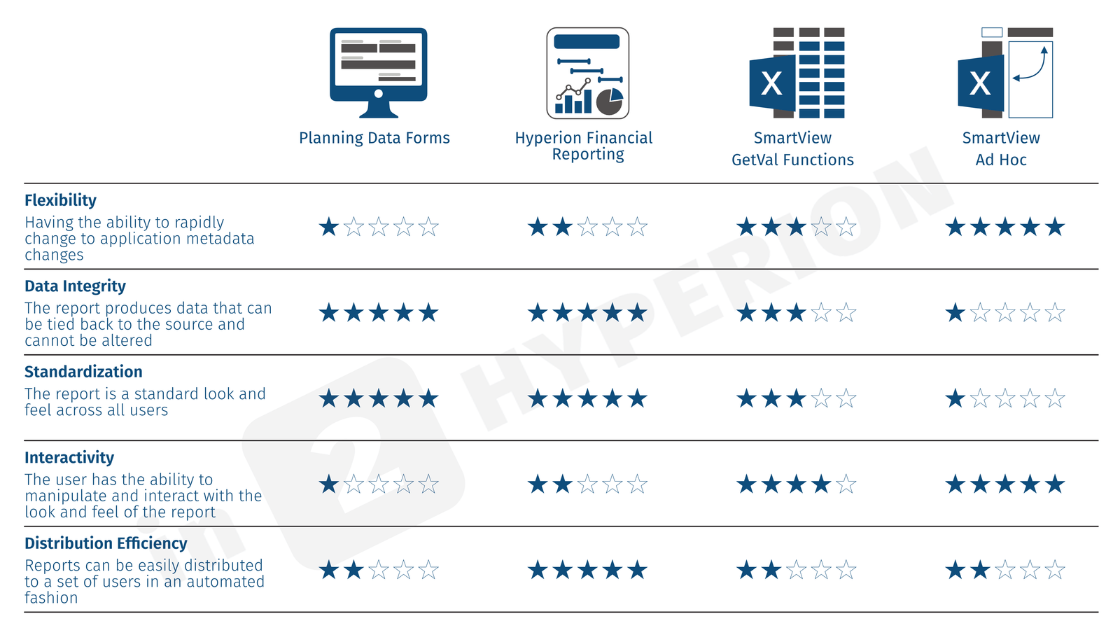
Planning Data Loads: com.hyperion.planning.InvalidMemberException vs. java.lang.RuntimeException

I had a very interesting thing happen today that tripped me up.  When loading data to a PBCS database through Planning (not as an Essbase file), I had two types of errors.  I have never seen this before and this could cause some serious heartburn for administrators and possibly waste a ton of time trying to resolve.  So, I am sharing for the sake of saving somebody some effort.

One Error, Two Messages

The error first is the typical error due to a member not being in the application.  com.hyperion.planning.InvalidMemberException: The member CTR_123 does not exist for the specified cube or you do not have access to it.  We have all seen this.  CTR_123 was not in the hierarchy.  Once it was added and the data was reloaded the issue was resolved.

The second issue was another error I have seen before, but I haven’t seen this in PBCS.  java.lang.RuntimeException: Not all dimensions were specified.  Normally, this is related to having a file correctly formatted in but having a member from one dimension in the wrong column, or having a column that is null.

As I often do, I created a Smart View retrieve and added the members in the load file one at a time.  When I found the member that caused a retrieve error, I went into the dimension editor to search for it.  To my surprise, it was there!  What?  But, when I looked at the properties, it was not valid for the application I was trying to load the data to.  This might have been overlooked by mere mortal (wink), but once enabled for the application in question, the load error was resolved.

Conclusion

So, why the two error types?  Why do we get two error types for the same error (the member doesn’t exist in the database)?  I can only assume since I loaded this through Planning, it tripped up on the fact that the member was in Planning, but not in the specific database I was trying to load.  If I loaded this as an Essbase file, as expected, I got the same error for both lines, member not found.

Hopefully this saves you some time.  If you have ever come across something similar, please share with the community.  These things are normally the things you find after a 12 hour day and you spend another 4 trying to figure it out.

Lastly, please enjoy a safe holiday and remind yourself how lucky you are and try to be thankful for the things you have and not be frustrated about the things you don’t.  Gobble Gobble!


Adventures in Groovy – Part 20: Groovy On-Premise vs. Groovy Cloud

Introduction

Yes, it is true that Groovy is available in on-premise and cloud (PBCS) versions of Hyperion Planning.  No, it is not true that the same flavor of Groovy exists in both.  Both have their advantages, and both have their drawbacks.  The likelihood that they will ever be the same is extremely low, and here is why.

The Difference Is

On-Premise gives developers the ability to write and use independent Groovy compiled applications.  These can be used in Business Rules as CDFs (custom defined functions).  Developers have complete functionality to make this do whatever they want.  It can return results to save to Essbase/Planning, it can interact with SQL, can run other programs, pretty much anything you can access that has a JAVA API.

PBCS doesn’t have the same flexibility.  Custom defined functions can’t be compiled and stored on the server.  PBCS, rather, has “Groovy Calculations.”  This gives developers the flexibility to interact with the Data Forms that on-premise doesn’t have.  Developers can iterate through the cells and act accordingly.  It can stop the form from saving, calculate and override data entered, color code cells, customize Data Maps, Smart Pushes, dynamically generate calculations, move data between databases, all with access to much of the Groovy functionality.

PBCS also supports the REST API, so Groovy can be used to access that and do everything, even more, that EPM Automate can do.

Why They Will Never Be The Same

This is just an opinion.  Technology changes so rapidly that this may change.  Corporate strategy changes almost as rapidly.

If PBCS had to ability to do what on-premise does, the ability for Oracle to support the instance would be a challenge.  CDFs can delete all the files on a server, for instance, and I don’t see a cloud provider giving developers this much control in a shared environment.

I also don’t see on-premise to have the same proactive interaction that PBCS has with Groovy Calculations purely because Oracle is pushing the cloud, and they want the most current functionality to exist in the platform they are pushing clients to use.

My Two Cents

I understand why there is a difference, and I don’t expect it to change in the near future.  3 years ago I didn’t expect that I would tell you that I would rather do a cloud implementation than on prem, either.  I do think as people get more comfortable with the cloud, and security improves, there will be advances.  I think there will be a future state where the cloud offerings will be closer to having the flexibility to the on-premise implementations.


Exporting Data in PBCS With Business Rules

Introduction

If your environment is a cloud product, whether it be PBCS or ePBCS, one thing that is critical to understand is the backups produced in the Migration area, may not be what you think.  Learning this after the fact may have negative consequences on your ability to restore data.  In the migration, the Essbase Data section is a copy of the pag, ind, and otl files.  When this is used to restore data, it restored the entire database.  This includes data and metadata.  This may be OK for many situation, but it won’t help you if

  • only specific data is required to be restored
  • specific data has changed and needs to be excluded from the restore
  • corruption exists in the database and all data is required to be restored
  • The pag files that hold the data are not readable
  • The size of the backup is quite large as it includes all data, and upper level data is normally exponentially larger than just level 0 data

Text Data Export

Business Rules can be written to export data to the Inbox/Outbox that is delimited with a few formatting options.  The entire database can be included.  With fix statements, specific data can be isolated.  So, forecast could be exported to a file, plan another, and actuals a third.  Specific accounts, entities, and/or products can be isolated in cases when specific data was inadvertently changed or deleted.  This file is a text file that can be opened in any text editor, Microsoft Excel, a database, or any other application that you open text files to view or manipulate.

Example Business Rule

/* Set the export options */
 SET DATAEXPORTOPTIONS
 {
 DataExportLevel LEVEL0;
 DataExportDynamicCalc OFF;
 DataExportNonExistingBlocks OFF;
 DataExportDecimal 4;
 DataExportPrecision 16;
 DataExportColFormat ON;
 DataExportColHeader Period;
 DataExportDimHeader ON;
 DataExportRelationalFile ON;
 DataExportOverwriteFile ON;
 DataExportDryRun OFF;
 };
 
 FIX(@Relative("Account", 0),
     @Relative("Years", 0),
     @Relative("Scenario", 0),
     @Relative("Version", 0),
     @Relative("Entity", 0),
     @Relative("Period", 0), 
     @Relative("custom_dim_name_1", 0),
     @Relative("custom_dim_name_1", 0),
     @Relative("custom_dim_name_1", 0))

  DATAEXPORT "File" "," "/u03/lcm/filename_xyz.txt" "";

 ENDFIX

Some Hints

There are a few things that you may encounter and be a little confused about, so the following are a few things that might help.

  1. To see the data export, it must be exported to /u03/lcm/, which is the equivalent of your inbox.  Any file name can be used.
  2. Setting DataExportLevel to 0 will export the level 0 blocks, not the level 0 members.  If there are any stored members in any of your dense dimensions, they will be exported unless the dimension is also in the fix to include ONLY level 0 members.
  3. The fix statement works the same as a fix statement in any business rule, so the data to be exported can be easily defined.
  4. My experience exporting dynamic calculated members drastically increases the time of the export.
  5. The export options are all pretty logical.  Some work in conjunction with each other and others are ignored depending on dependent setting values.  These are documented for version 11.1.2.4 here.
  6. This process can be automated with EPM Automate and include the download and time stamp of the backup for later use.

Conclusion

There are benefits to both types of backups.  My preference is to either run both nightly, or run just the Business Rule.  By having both, the administrator has the option of restoring the data as needed, in the way that is most effective.  Having both provides the ultimate flexibility.  If space is an issue, exclude the data option in the Migration and just run the business rule.


From Oracle’s Documentation

DataExportLevel ALL | LEVEL0 | INPUT

  • ALL—(Default) All data, including consolidation and calculation results.
  • LEVEL0—Data from level 0 data blocks only (blocks containing only level 0 sparse member combinations).
  • INPUT—Input blocks only (blocks containing data from a previous data load or grid client data-update operation). This option excludes dynamically calculated data. See also the DataExportDynamicCalc option.

In specifying the value for the DataExportLevel option, use these guidelines:

  • The values are case-insensitive. For example, you can specify LEVEL0 or level0.
  • Enclosing the value in quotation marks is optional. For example, you can specify LEVEL0 or “LEVEL0”.
  • If the value is not specified, Essbase uses the default value of ALL.
  • If the value is incorrectly expressed (for example, LEVEL 0 or LEVEL2), Essbase uses the default value of ALL.

Description

Specifies the amount of data to export.

DataExportDynamicCalc ON | OFF

  • ON—(Default) Dynamically calculated values are included in the export.
  • OFF—No dynamically calculated values are included in the report.

Description

Specifies whether a text data export excludes dynamically calculated data.

Notes:

  • Text data exports only. If DataExportDynamicCalc ON is encountered with a binary export (DATAEXPORT BINFILE …) it is ignored. No dynamically calculated data is exported.
  • The DataExportDynamicCalc option does not apply to attribute values.
  • If DataExportLevel INPUT is also specified and the FIX statement range includes sparse Dynamic Calc members, the FIX statement is ignored.

DataExportNonExistingBlocks ON | OFF

  • ON—Data from all possible data blocks, including all combinations in sparse dimensions, are exported.
  • OFF—(Default) Only data from existing data blocks is exported.

Description

Specifies whether to export data from all possible data blocks. For large outlines with a large number of members in sparse dimensions, the number of potential data blocks can be very high. Exporting Dynamic Calc members from all possible blocks can significantly impact performance.

DataExportPrecision n

n (Optional; default 16)—A value that specifies the number of positions in exported numeric data. If n < 0, 16-position precision is used.

Description

Specifies that the DATAEXPORT calculation command will output numeric data with emphasis on precision (accuracy). Depending on the size of a data value and number of decimal positions, some numeric fields may be written in exponential format; for example, 678123e+008. You may consider using DataExportPrecision for export files intended as backup or when data ranges from very large to very small values. The output files typically are smaller and data values more accurate. For output data to be read by people or some external programs, you may consider specifying the DataExportDecimal option instead.

Notes:

  • By default, Essbase supports 16 positions for numeric data, including decimal positions.
  • The DataExportDecimal option has precedence over the DataExportPrecision option.

Example

SET DATAEXPORTOPTIONS
    { 
    DataExportPrecision 6;
    DataExportLevel ALL;
    DataExportColHeader "Measures";
    DataExportDynamicCalc ON;
    };
    DATAEXPORT "File" "," "output1.out";

Initial Data Load Values

"Sales" "COGS" "Margin" "Marketing" "Payroll" "Misc" "Total Expenses" "Profit" "Opening Inventory" "Additions" "Ending Inventory" "Margin %" "Profit %" 
"100-10" "New York"
"Jan" "Actual" 678123456.0 271123456.0 407123456.0 941234567890123456.0 51123456.0 0 145123456.0 262123456.0 2101123456.0 644123456.0 2067123456.0 60123456.029 38123456.6430
"Feb" "Actual" 645123 258123 3871234 9012345 5112345 112345678 14212345 24512345 2067123456 61912345 20411234 601234 37123456.98 
"Mar" "Actual" 675 270 405 94 51 1 146 259 2041 742 2108 60 38.37037037037037 
"Qtr1" "Actual" 1998 799 1199 278 153 2 433 766 2101 2005 2108 60.01001001001001 38.33833833833834

Exported Data Format

"Sales","COGS","Margin","Marketing","Payroll","Misc","Total Expenses","Profit","Opening Inventory","Additions","Ending Inventory","Margin %","Profit %","Profit per Ounce","100-10","New York"
"Jan","Actual",6.78123e+008,2.71123e+008,4.07e+008,9.41235e+017,5.11235e+007,0,9.41235e+017,-9.41235e+017,2.10112e+009,6.44123e+008,2.06712e+009,60.0186,-1.388e+011,-7.84362e+016
"Feb","Actual",645123,258123,387000,9.01235e+006,5.11235e+006,1.12346e+008,1.2647e+008,-1.26083e+008,2.06712e+009,6.19123e+007,2.04112e+007,59.9886,-19544.1,-1.05069e+007
"Mar","Actual",675,270,405,94,51,1,146,259,2041,742,2108,60,38.3704,21.5833

DataExportDecimal n

Where n is a value between 0 and 16.

If no value is provided, the number of decimal positions of the data to be exported is used, up to 16 positions, or a value determined by the DataExportPrecision option if that is specified.

Description

Specifies that the DATAEXPORT calculation command will output numeric data with emphasis on legibility; output data is in straight text format. Regardless of the number of decimal positions in the data, the specified number is output. It is possible the data can lose accuracy, particularly if the data ranges from very large values to very small values, above and below the decimal point.

Notes:

  • By default, Essbase supports 16 positions for numeric data, including decimal positions.
  • If both the DataExportDecimal option and the DataExportPrecision option are specified, the DataExportPrecision option is ignored.

Example

SET DATAEXPORTOPTIONS
    {DataExportDecimal 4;
    DataExportLevel "ALL";
    DataExportColHeader "Measures";
    DataExportDynamicCalc ON;
    };
    DATAEXPORT "File" "," "output1.out";

Initial Data Load Values

"Sales" "COGS" "Margin" "Marketing" "Payroll" "Misc" "Total Expenses" "Profit" "Opening Inventory" "Additions" "Ending Inventory" "Margin %" "Profit %" 
"100-10" "New York"
"Jan" "Actual" 678123456.0 271123456.0 407123456.0 941234567890123456.0 51123456.0 0 145123456.0 262123456.0 2101123456.0 644123456.0 2067123456.0 60123456.029 38123456.6430
"Feb" "Actual" 645123 258123 3871234 9012345 5112345 112345678 14212345 24512345 2067123456 61912345 20411234 601234 37123456.98 
"Mar" "Actual" 675 270 405 94 51 1 146 259 2041 742 2108 60 38.37037037037037 
"Qtr1" "Actual" 1998 799 1199 278 153 2 433 766 2101 2005 2108 60.01001001001001 38.33833833833834

Exported Data Format

"Sales","COGS","Margin","Marketing","Payroll","Misc","Total Expenses","Profit","Opening Inventory","Additions","Ending Inventory","Margin %","Profit %","Profit per Ounce"
"100-10","New York"
"Jan","Actual",678123456.0000,271123456.0000,407000000.0000,941234567890123520.0000,51123456.0000,0.0000,941234567941246980.0000,-941234567534246910.0000,2101123456.0000,644123456.0000,2067123456.0000,60.0186,-138799883591.4395,-78436213961187248.0000
"Feb","Actual",645123.0000,258123.0000,387000.0000,9012345.0000,5112345.0000,112345678.0000,126470368.0000,-126083368.0000,2067123456.0000,61912345.0000,20411234.0000,59.9886,-19544.0820,-10506947.3333
"Mar","Actual",675.0000,270.0000,405.0000,94.0000,51.0000,1.0000,146.0000,259.0000,2041.0000,742.0000,2108.0000,60.0000,38.3704,21.5833

Output Format Options

DataExportColFormat ON | OFF

  • ON—The data is output in columnar format.
  • OFF—Default. The data is output in non-columnar format.

Description

Specifies if data is output in columnar format. Columnar format displays a member name from every dimension; names can be repeated from row to row, enabling use by applications other than Essbase tools. In non-columnar format, sparse members identifying a data block are included only once for the block. Non-columnar export files are smaller, enabling faster loading to an Essbase database.

Notes

Do not use the DataExportColFormat option in combination with the DataExportRelationalFile option, which already assumes columnar format for files destined as input files to relational databases.

Example

SET DATAEXPORTOPTIONS
 {
 DATAEXPORTCOLFORMAT ON;
 };
 FIX("100-10", Sales, COGS, Jan, Feb, Mar, Actual, Budget)
 DATAEXPORT "File" "," "d:\temp\test2.txt" ;
ENDFIX;

DataExportColHeader dimensionName

Description

Specifies the name of the dense dimension that is the column header (the focus) around which other data is referenced in the export file. Use the DataExportColHeader option only when you export data to a text file. For example, if from Sample Basic the Year dimension is specified, the output data starts with data associated with the first member of the Year dimension: Year. After all data for Year is output, it continues with the second member: Qtr1, and so on.

Notes

MaxL, ESSCMD, and Essbase exports do not provide a similar capability. With these methods, Essbase determines the focal point of the output data.

Exporting through Report Writer enables you to specify the header in the report script.

Example

SET DATAEXPORTOPTIONS {DATAEXPORTCOLHEADER Scenario;};

Specifies Scenario as the page header in the export file. The Scenario dimension contains three members: Scenario, Actual, and Budget. All Scenario data is shown first, followed by all Actual data, then all Budget data.

DataExportDimHeader ON | OFF

  • ON—The header record is included.
  • OFF—Default. The header record is not included.

Description

Use the DataExportDimHeader option to insert the optional header record at the beginning of the export data file. The header record contains all dimension names in the order as they are used in the file. Specifying this command always writes the data in “column format”.

Example

SET DATAEXPORTOPTIONS 
 {
 DATAEXPORTLEVEL "ALL"; 
 DATAEXPORTDIMHEADER ON; 
 };
FIX("100-10", "New York", "Actual")
 DATAEXPORT "File" "," "E:\temp\2222.txt" ;
ENDFIX;

Specifying the DataExporttDimHeader ON option while exporting Sample Basic writes the data in column format, with common members repeated in each row. The data begins with a dimension header, as shown in the first two rows of the example file below:

"Product","Market","Year","Scenario","Measures"
"Sales","COGS","Marketing","Payroll","Misc","Opening Inventory","Additions","Ending Inventory"
"100-10","New York","Jan","Actual",678,271,94,51,0,2101,644,2067
"100-10","New York","Feb","Actual",645,258,90,51,1,2067,619,2041
"100-10","New York","Mar","Actual",675,270,94,51,1,2041,742,2108
"100-10","New York","Apr","Actual",712,284,99,53,0,2108,854,2250
"100-10","New York","May","Actual",756,302,105,53,1,2250,982,2476
"100-10","New York","Jun","Actual",890,356,124,53,0,2476,1068,2654
"100-10","New York","Jul","Actual",912,364,127,51,0,2654,875,2617
"100-10","New York","Aug","Actual",910,364,127,51,0,2617,873,2580
"100-10","New York","Sep","Actual",790,316,110,51,1,2580,758,2548
"100-10","New York","Oct","Actual",650,260,91,51,1,2548,682,2580
"100-10","New York","Nov","Actual",623,249,87,51,0,2580,685,2642
"100-10","New York","Dec","Actual",699,279,97,51,1,2642,671,2614

DataExportRelationalFile ON | OFF

  • ON—The output text export file is formatted for import to a relational database.
    • Data is in column format; sparse member names are repeated. (The DataExportColFormat option is ignored.)
    • The first record in the export file is data; no column heading or dimension header is included, even if specified. (The DataExportColHeader and DataExportDimHeader options are ignored.)
    • Missing and invalid data is skipped, resulting in consecutive delimiters (commas) in the output. The optional “missing_char” parameter for DATAEXPORT is ignored
  • OFF—Default. The data is not explicitly formatted for use as input to a relational database.

Description

Using the DataExportRelationalFile option with DATAEXPORT enables you to format the text export file to be used directly as an input file for a relational database.

Example

SET DATAEXPORTOPTIONS {
 DataExportLevel "ALL";
 DataExportRelationalFile ON;
};

FIX (Jan)
 DATAEXPORT "File" "," c:\monthly\jan.txt
ENDFIX;

Processing Options

DataExportOverwriteFile ON | OFF

  • ON—The existing file with the same name and location is replaced.
  • OFF—Default. If a file with the same name and location already exists, no file is output.

Description

Manages whether an existing file with the same name and location is replaced.

DataExportDryRun ON | OFF

  • ON—DATAEXPORT and associated commands are run, without exporting data.
  • OFF—Default. Data is exported

Description

Enables running the calculation script data export commands to see information about the coded export, without exporting the data. When the DataExportDryRun option value is ON, the following information is written to the output file specified in the DATAEXPORT command:

  • Summary of data export settings
  • Info, Warning, and Error messages
  • Exact number of blocks to be exported
  • Estimated time, excluding I/O time.

Notes

  • The DataExportDryRun option does not work with exports to relational databases.
  • If you modify the script for reuse for the actual export, besides removing the DataExportDryRun option from the script you may want to change the name of the export file.

Example

SET DATAEXPORTOPTIONS 
 {
 DataExportLevel "ALL";
 DataExportColHeader "Measures";
 DataExportColFormat ON;
 DataExportDimHeader ON;
 DataExportDynamicCalc OFF;
 DataExportDecimal 0;
 DataExportDryRun ON;
 DataExportOverwriteFile ON;
 };

FIX("Qtr1")
 DATAEXPORT "File" "," "E:\temp\log.txt" ;
ENDFIX;


Adventures in Groovy – Part 3: Acting On Edited Cells

Introduction

With the introduction of Groovy Calculations this summer, one of the things I use most, especially for applications with data forms that include a large sparse dimension in the rows with suppression on, is the option to loop through cells and identify only the POV on the cells that have changed.  In applications like workforce planning, or product level applications that have hundreds, if not thousands, of possible blocks, isolating only the changed data can have significant impacts on performance.  Normally when a data form is saved, the fix includes all level 0 members of the employee dimension and must run the calculations on all of them, regardless of whether employee changed or not.  Being able to fix on only a row, or the handful that change, give us a significant advantage in user response.

This post will go into how this is executed, and a few use cases to get you thinking about the possibilities.  All of these I have developed and are in a production application.

The Code

Using a grid iterator, with the appropriate parameter, is an extremely easy way to deploy functionality that looks through ONLY the cells that have been changed.

 operation.grid.dataCellIterator({DataCell cell -> cell.edited}).each{
  [actions]
 }

The cell object, and all its parameters, are available inside the loop.  By adding {DataCell cell -> cell.edited}, the loop is isolated to only cells that have changed.  The representative member names, the data value, if it is locked, has attachments, and many other things can be accessed with the example above.

Use Cases

An infinite number of uses are possible, as you are probably already thinking about. If not, the following will probably spark some creativity.

Customizing an Essbase Fix Statement

One of the most significant benefits of this is the ability to be able to dynamically generate a fix statement and filter what is calculated.  Although the calculation on the Essbase side isn’t improved just by using Groovy, the ability to dynamically write the calculation on only what changed is significant, especially when allocations, data pushes, and other longer running processes are required.

Assuming the rows of a data grid include the dimension Product, and Period is in the columns, the following will create variables that will include only the periods and products that have been updated.  These can be used in the string builder that is passed to Essbase.  So, rather than @RELATIVE(“Product”,0) running on all possible products, it can be replaced with “Product 1″,”Product 2”.

The following creates list and string variable for Product and Period.  Every cell that is updated will add the relative product and period to the list variables.  After all the cell values have been read, the two string variables are set to include a unique list of the dimension members, surrounded by quotes, and separated by commas, which are immediately ready to include in the FIX statement.

def lstProducts = []
def lstPeriods = []
operation.grid.dataCellIterator({DataCell cell -> cell.edited}).each{
  lstProducts.add(it.getMemberName("Product"))
  lstPeriods.add(it.getMemberName("Period"))
  }
def strProducts = '"' + lstProducts.unique().join('","') + '"'
def strPeriods = '"' + lstPeriods.unique().join('","') + '"'

The string builder would look something like this.  In the following example, the other variables are pulled from the POV.

def sScenario=povmbrs.find {it.dimName =='Scenario'}.essbaseMbrName
def sCompany=povmbrs.find {it.dimName =='Company'}.essbaseMbrName
def sYear=povmbrs.find {it.dimName =='Year'}.essbaseMbrName

StringBuilder strEssCalc = StringBuilder.newInstance()
strEssCalc <<"""FIX($sScenario,
  $sCompany,
  $sYear,
  $strProducts,
  $strPeriods
)
 Revenue = units * price;
ENDFIX
"""

At this point, the strEssCalc value can be passed to Essbase and executed.  If only 2 products are changed in 1 month, only those 2 cells would be calculated.  If this data form included 12 months and 1,000 products, the calculation would take roughly 1/500th of the time.

Customizing Smart Push

Smart Pushes on forms, depending on the POV, can exceed a threshold of what a user perceives as acceptable performance.  In the 17.11 release, Data Maps and Smart Pushes can now embedded in the Groovy Calculations.  The 2 huge benefits to this are that

  1. the data that is pushed can be filtered to only the data that changes, decreasing the time of the operation, and
  2. the ability control the operation order of when a push runs (for example, calculation, push, calculation, push)

If a data form has a smart push associated to it, it can be accessed and further customized.  If not, data maps can also be accessed, customized, and executed.

One thing I learned from the Oracle development team is that the Smart Pushes have a max memory that can be accessed.  One Smart Push may never hit that limit if it is isolated enough, but we found issues when multiple Smart Pushes were executed a the same time.  We were seeing multiple, and intermediate, failures in the logs.  So, it is even more critical to make these pushes as small as possible to eliminate that issue.

If we reference the example above in the customized fix, we expand on that and apply the same filter to the Smart Push.  The only addition needed is to encapsulate the strProducts variable in quotes.  If nothing is passed, it runs the smart push as it is setup in the form, so operation.grid.getSmartPush(“appname”).execute() would simply execute the same thing as if the Smart Push was set to run on save.

strProducts = """ + strProducts + """
if(operation.grid.hasSmartPush("appname"))
  operation.grid.getSmartPush("appname").execute(["Product":strProducts,"Period":strPeriods])

Validate data

Having the ability to proactively perform data validation is another great addition with Groovy.  Rather than running a calculation, and after the Data Form save returning a message telling the user that they have to change something, or changing it for them, we now can interrupt the data form save and instruct the user to change it before it has any adverse impact on the data.  The following will change the cells that violate the validation to red, add a tooltip, stop the form save, and throw an error message.  Assume we don’t want the user to enter more than 50,000 in salary.  This threshold can point to data in the application, but is hard coded below for simplicity.

operation.grid.dataCellIterator({DataCell cell -> cell.edited}).each{ 
  if(it.data > 50000){
    it.addValidationError(0xFF0000, "Salary is outside of the allowed range.")
  }
}

Conclusion

This is just a taste of what can be done.  As you can see, with the ability to isolate actions on only the dirty cells, we now have opportunities we haven’t had since pre Smart View, and functions are completely new.  The impact on performance is game changing and the ability we now have to interact with a user pre and post save is ground breaking to the possibilities.


Choosing a Reporting Mechanism in Planning

Reports out of Hyperion Planning are typically identified in 2 categories.

  • Standard “canned” reports – These reports are used generically in a global aspect to report data in common formats and standardized views. These are often generated in volume and printed for presentations and executive review.
  • Ad hoc reports – These reports are more flexible, often adjusted to explain current variances and market conditions. These reports are most likely generated by analysts and managers producing unique views to explain variances that exist at a point in time.  The need to alter, change, and customize these reports are essential to identify and explaining current business conditions.

Reporting from Hyperion Planning can be completed in 3 (debatably 4) ways.  Deciding which reports are developed, or produced, and in which delivery method, is critical to making the most of the reporting capabilities and development time available.

The recommended approach for reports that are distributed globally, need to have a consistent look and feel, and use standard hierarchies and financial definitions, is to build them in Hyperion Financial Reporting. This will enable users to execute the exact same report, with their specific point of view, and distribute it to anybody in the company.  It can also be mass distributed by email to thousands of users for their specific business ownership when data is finalized.  Reports can be grouped into books so users can easily run a set of reports for their line of business quickly and easily. Development of reports in HFR take a little longer are can be more time consuming to change, so selecting reports in this delivery method should be evaluated and considered carefully.

Reports that consistently change, are not required to be mass produced, or don’t require a defined format, are more commonly produced in SmartView/Excel.  This delivery method provides the ultimate flexibility in creativity and customization.  These reports can be rapidly produced and development and is cost effective.  These reports, although extremely flexible, require complete ownership on data validation by the users, as they don’t change automatically to the changes in the hierarchies of the application.  Developing reports in SmartView/Excel is extremely beneficial when the report changes rapidly and it supports the ability to quickly identify business variances and explain those variances to management.

The following matrix will help you identify the best reporting method for your environment.


My Adventures in Groovy Calculations – Part 1

What Is Groovy

Recently, Groovy scripting was added to ePBCS business rules as an option instead of the GUI, or the go-to scripting for you old-timers who still refuse to change.  These are defined in the Business Rule editor as Groovy calculations.  So, what is Groovy?

“Apache Groovy is an object-oriented programming language for the Java platform. It is a dynamic language with features similar to those of Python, Ruby, Perl, and Smalltalk. It can be used as a scripting language for the Java Platform, is dynamically compiled to Java virtual machine (JVM) bytecode, and interoperates with other Java code and libraries. Groovy uses a Java-like curly-bracket syntax. Most Java code is also syntactically valid Groovy, although semantics may be different.”

If you haven’t heard of Groovy, you may want to do some research.  Oracle is using more and more Groovy in applications as administrative options and a communication method between applications.  Groovy is a standard and can be used with millions of applications and websites with the REST API.

What Groovy Script/Calculations Are Not

Groovy calculations are not java-based calculations.  It is not a new calculation language.  It does provide a way to interact with a Data Form in ePBCS and build a calculation script dynamically.  So, Groovy, in the context of Groovy Calculation Scripts, does not connect to Essbase via Groovy Business Rules. It simply builds a string that is sent to Essbase as a calculation.  It does, however, interact with Planning and that is where the power starts.  With the ability to have all the Groovy functionality to manipulate strings and now the ability to interact with the data form, dynamic calculations can be built.  The calculation script sent to Essbase is no different, but the script can now be dynamically generated based on things like, the POV, the text value of a Smart List, whether the values in the grid were updated, whether the data entered meets validation criteria, and other similar things.

If you are experienced with Hyperion Planning, you may have dabbled with JavaScript to do data validation, calculate data prior to the user submitting it, or prevent users from submitting data.  It was a great option to provide feedback to users, but that basically was useless when Smart View allowed users to open Data Forms in Excel. The JavaScript did nothing unless the form was opened in an internet browser.

Getting Started

The first step in creating a Groovy Calculation Script is to, well, create one.  To do that, create a new business ruleChange the view from Designer to Edit Script.  If you haven’t noticed this before, it provides a way to toggle the GUI to a script view.

Next, find the drop-down box in the toolbar to the far right named Script Type.  This option will read Calc Script.  Change it to Groovy Script.

AAt this point, the script window is now set to validate Groovy script, not Essbase syntax. Even though it doesn’t do anything yet, you have just created your first Groovy Business Rule!

Use Cases

There is a lot of potential in this functionality.  To get you thinking, here are some examples:

  1. Execute calculations on large sparse dimensions on ONLY the members that changed on the form.
  2. Access the Smart List text to do validation, use in calculations, and store for later use in Essbase (maybe save a member name in a member that is numeric, like employee ID, Cost Center, or account).
  3. Perform validation before the calculation is built and sent to Essbase. For example, if the sum of a column used to allocate dollars doesn’t sum to 100, send a calculation that ONLY returns a message and doesn’t perform the allocation.
  4. Perform text manipulation previously done in Essbase with functions.  Concatenating member names and truncating member name prefixes and date formats are some of the few I use regularly.  Many of these functions are extremely slow and force the calculation to execute in serial mode, so to be able to do them outside the script is now an option.

Real World Example

The Problem

I am working with a client who wants to override the result of driver-based calculations based on historical trends.  In this example, the volume of cases can be changed and the profit rate can be adjusted.  Once the form is saved, the overrides need to be removed.

Here-in lies the challenge.  If the overrides are removed and the calculation runs on all members in the form, the results would revert back to what they were prior to the override because the override values no longer exist in the database or Data Form.  So, rather than perform the calculation on the override, it would use #missing  or zero, and take the results right back to what the drivers dictated.  The most obvious way around this issue is to execute the calculation on ONLY the rows (vendors in this example) that were edited. In other words, dynamically generate the FIX statement on the vendors that were updated.

The Non-Groovy FIX Statement

Without Groovy, the FIX statement would include @RELATIVE(“Vendor”,0) to run the calculation on all venders on the Data Form.  This has 2 issues.  One, it calculates all the vendors and will change the vendors back to the pre-override values.  Two, every time the user saves the form, the fix is traversing through 30,000 possible vendors.  Although most companies have less than 8,000 active vendors, it still poses a performance issue calculating 8,000 blocks when only a few typically change.

The only aspect of the calculation that is going to change in this situation is the FIX statement, so that will be the only piece shown in the comparison between a Groovy script and a non-Groovy script.

FIX(&vScenario,
    &vVersion,
    &vCompany,
    &vYear,
    "Local",
    "Input",
    @RELATIVE(“Vendor”,0),
    "Jan":"Dec",
    "Regular_Cases")

The Groovy FIX Statement

Since Groovy can dynamically create the calculation script, it looks more like the example below. The sPov will be a string variable in Groovy that holds all the members in the data form’s POV.  The sVendors Groovy variable will hold the list of vendors that have been edited.

FIX($sPOV
    $sVendors,
    "Jan":"Dec",
    "Regular_Cases")

@RELATIVE(“Vendor”,0), which would produce a list of every vendor in the hierarchy, is replaced with “V300000300040003”, “V300000300060001”, “V300000300070002”.

The issue of running the calculation on vendors that have not been edited has now been solved.  An added benefit is that the calculation runs on 3 of the 8,000 blocks, so what took 30 seconds now completes in under a second.

Now, The Interesting Part

Let’s dissect the Groovy calculation script piece by piece.

Setting The Stage

For Groovy to perform operations, there are a few housekeeping items that need to be addressed.  First, a few string builders need to be created to store some variables of strings that grow through the process and are concatenated to Essbase calculation before it is submitted for processing.

There are some variables used to interact with the form’s data grid.  For easy reference to the grid through the script, the grid object is stored in a variable (curgrid).  Next, a variable is created to hold the result of the cells that have been edited (itr).    The likelihood that these variables would exist in most of the scripts is high, so it might make sense to get familiar with these objects and their parameters.

//Get current Data Form
DataGrid curgrid = operation.getGrid()

// Construct a string builder
// Holds the calculation script sent to Essbase
StringBuilder scriptBldr = StringBuilder.newInstance()

// Holds the value for the venders that have changed
StringBuilder vendorList = StringBuilder.newInstance()
String sVendors

// Iterater which gives you only the edited cells
GridIterator itr = curgrid.getDataCellIterator(PredicateUtils.invokerPredicate("isEdited"))

// Holds the list of members from the POV – the function returns an array, so this
// parsed the array and places quotes around each member and separates them with a comma
String sPov = '"' + curgrid.getPov().essbaseMbrName.join(',').replaceAll(',','","') + '"'

At this point the values of the variables are as follows.

Find the Vendors That Have Changed

We know the users will enter overrides in this Data Form (Case Growth and Average Price).  The following piece of the Groovy script will build a delimited list of those vendors based on the rows that have been edited.  It will include quotes around the member names to account for any member names that are numeric or have special characters and will be separated by a comma.  Groovy provides the ability to append to a string with <<”””, and close it with “””.  The if statement ensures that a vendor will not be appended to the string if multiple columns are changed.

// Loop through each cell that was edited and build the vendor list
// If multiple cells on the same row are edited, only add vendor once
itr.each{ DataCell cell ->
  sVendors = cell.getMemberName("Vendor")
  if(vendorList.indexOf(sVendors) < 0){
    vendorList <<"""
   ,"$sVendors"
   """
  }
}

At this point, only a few variables have changed. The bulk of the Groovy functionality is finished.  We now have the POV and the list of vendors that need to be in the FIX statement.

The Essbase Calculation

The next section will append text to the scriptBldr string.  This string will ultimately be sent to Essbase as the calculation to be performed.  Groovy variables are embedded and replaced with the value that they were set to previously.  The two used in this calculation are $vendorList and $sPOV.  Other than those two pieces, everything else is pulled from the original Business Rule and highlighted in red below.

// Add the calculation defined in a business rule to the string variable
// the POV and Vendor List will be used to dynamically set the FIX statement
scriptBldr <<"""
VAR v_Price;

FIX($sPOV
    $vendorList,
    "Jan":"Dec",
    "Regular_Cases")

  /* Calculate Overrides */
  "OEP_Working"(
  v_Price = "Avg_Price/Case"->"YearTotal";

  "Regular_Cases" = (1 + "Case_Growth_Rate"->"BegBalance") * 
                    ("Regular_Cases"->"FY16"->"Final");
  IF("Avg_Price/Case_Inp"->"BegBalance" == #Missing)
    "Net_Sales" = (v_Price) * (1 + "Case_Growth_Rate"->"BegBalance") * 
                  "Regular_Cases"->"FY16"->"Final";
  ELSE
    "Net_Sales" = ("Avg_Price/Case_Inp"->"BegBalance") * 
                  (1 + "Case_Growth_Rate"->"BegBalance") *
                  "Regular_Cases"->"FY16"->"Final" ;
  ENDIF

  IF("GP_2_%_Inp"->"BegBalance" == #Missing)
    "GP_Level_2" = ("GP_Level_2_%"->"YearTotal"->"FY16"->"Final") * "Net_Sales" ;
  ELSE
    "GP_Level_2" = ("GP_2_%_Inp"->"BegBalance") * "Net_Sales" ;
  ENDIF
  )
ENDFIX

FIX($sPOV
    $vendorList)

  CLEARDATA "Avg_Price/Case_Inp"->"BegBalance";
  CLEARDATA "GP_2_%_Inp"->"BegBalance";
  CLEARDATA "Case_Growth_Rate"->"BegBalance";
ENDFIX
"""

At this point, the scriptBldr variable is a complete Essbase calculation that can be validated in any Business Rule.

Finishing UP

The last thing required is to send the calculation text built above to Essbase.

println scriptBldr // Sends the script to the log
return scriptBldr // Sends the script to Essbase

Verifying What Was Sent To Essbase

When the Data Form is saved, the results in the form can be validated back to the logic to verify that the calculation worked as expected.  Regardless of whether the calculation executes with or without failing, the value of scriptBldr ( calculation sent to Essbase) is captured in the Job console.

In the Job console, click the Job Status link.  This includes the value of the scriptBldr variable.  The text can be copied from this window, and if it failed to execute, can be copied into a Business Rule and validated there to find the issue.

Wrapping Up

I will admit that I am not a Java programmer, so I am still educating myself on the potential this affords developers.  I am struggling to digest the API documentation and to truly understand the depth of the possibilities. I do know this opens up a whole world we didn’t have with Hyperion Planning. I plan on learning and using Groovy calculations more and more because of the possibilities it provides.  Look for more examples and knowledge sharing as I get my hands around the API and integrate this into more delivery solutions.  To get future publications, sign up to be notified about new posts and articles at www.in2hyperion.com.


Using a Shared Connection with HSGetValue/HSSetValue with Planning or PBCS

If you are a fan of the HSGetValue and HSSetValue, you probably are using a private connection. As you know, anybody that uses the template has to either change the connection string to their own predefined private connection, or set up a private connection with the same name. When dealing with inexperience users, both methods can be problematic.

You may be surprised to know that the Get and Set Value functions can use a shared connection. Rather than using the private connection name, the following can be specified to use a shared connection in place of the private connection name.

Private connection syntax:
HsGetValue(“PrivateConnectionName”,”POV”)
HsSetValue (dollar amount,”PrivateConnectionName”,”POV”)

Shared connection syntax:

HsGetValue(“WSFN|ProviderType|Server|Application|Database”,”POV”)
HsSetValue (dollar amount,”WSFN|ProviderType|Server|Application|Database”,”POV”)

Parameter Summary

  • “WSFN” is a static string and never changes
  • The provider type for planning is “HP” regardless of whether the server is a cloud server or on premise server
  • The server specifies the location of the server housing the application. For PBCS, use the URL provided by Oracle (planning-test-domain.pbcs.us2.oraclecloud.com)
  • The application is the application name
  • The database is the plan type, or database name

Put that all together and the string looks like this.
WSFN|HP|planning-test-A12345.pbcs.us2.oraclecloud.com|Finance|Revenue

Conclusion

Although there are a few drawbacks to using a shared connection (users could use the wrong connection and not get the expected result), my experience has been that the pros (no setup of private connections, can be used in multiple environments without changing anything, etc.) far outweigh the cons.


Remove Dimensions From Planning LCM Extracts

Problem

I am currently working with a client that is updating a planning application and one of the changes is to remove a dimension.  After the new application was setup and the hierarchies were modified to meet the objectives, migrating artifacts was the next step.  As many of you know, if you try to migrate web forms and composite forms, they will error during the migration due to the additional dimension in the LCM file.  It wouldn’t be a huge deal to edit a few XML files, but when there are hundreds of them, it is extremely time consuming (and boring, which is what drove me to create this solution).

Assumptions

To fully understand this article, a basic understanding of XML is recommended.  The example below assumes an LCM extract was run on a Planning application and it will be used to migrate the forms to the same application without a CustomerSegment dimension.  It is also assumed that the LCM extract has been downloaded and decompressed.

Solution

I have been learning and implementing PowerShell scripts for the last 6 months and am overwhelmed by how easy it is to complete complex tasks.  So, PowerShell was my choice to modify these XML files in bulk.

It would be great to write some long article on how smart this solution is and overwhelm you with my whit, but there is not much too it.  A few lines of PowerShell will loop through all the files and remove the XML tags related to a predefined dimension.  So, let’s get to it.

Step 1 – Understand The XML

There are two folders of files we will look to.  Forms are under the plan type and the composite forms are under the global artifacts.  Both of these are located inside the resource folder.  If there are composite forms that hold the dimension in question as a shared dimension, both will need to be impacted.  Scripts will be included to update both of these areas.

Inside each of the web form files will be a tag for each dimension, and it will vary in location based on whether the dimension is in the POV, page, column, or row.  In this particular example, the CustomerSegment dimension is in the POV section.  What we want to accomplish is removing the <dimension/> tag where the name attribute is equal to CustomerSegment.

For the composite forms, the XML tag is slightly different, although the concept is the same.  The tag in composite form XML files is <sharedDimension/> and the attribute is dimension, rather than name.

Step 2 – Breaking Down the PowerShell

The first piece of the script is just setting some environment variables so the script can be changed quickly so that it can be used wherever and whenever it is needed.  The first variable is the path of the Data Forms folder to be executed on.  The second is the dimension to be removed.

# Identify the source of the Data Forms folder and the dimension to be removed
# List all files, recursively, that exist in the path above
$files = Get-ChildItem $lcmSourceDir -Recurse | 
where {$_.Attributes -notmatch 'Directory'} |

The next piece of the script is recursing through the folder and storing the files in an array.  There is a where statement to exclude directories so the code only executes on files.

# List all files, recursively, that exist in the path above
$files = Get-ChildItem $lcmSourceDir -Recurse | 
where {$_.Attributes -notmatch 'Directory'} |
Step 3 – Removing The Unwanted Dimension

The last section of the script does most of the work.  This will loop through each file in the $files array and

  1. Opens the file
  2. Loops through all tags and deletes any <dimension/> tag with a name attribute with a value equal to the $dimName variable
  3. Saves the file
# Loop through the files and find an XML tag equal to the dimension to be removed
Foreach-Object {

$xml = Get-Content $_.FullName
$node = $xml.SelectNodes(“//dimension”) |
Where-Object {$_.name -eq $dimName} | ForEach-Object {
# Remove each node from its parent
[void][/void]$_.ParentNode.RemoveChild($_)
}
$xml.save($_.FullName)
Write-Host “($_.FullName) updated.”
}

Executing The Logic On Composite Forms

The above concepts are exactly the same to apply the same logic on composite forms files in the LCM.  If this is compared to the script applied to the web forms files, there are three differences.

  1. The node, or XML tag, that needs to be removed is called sharedDimension, not dimension. (highlighted in red)
  2. The attribute is not name in this instance, but is called dimension.  (highlighted in red)
  3. We have added a counter to identify whether the file has the dimension to be removed and only saves the file if it was altered.  (highlighted in green)
The Script
$lcmSourceDir = "Z:\Downloads\KG04\HP-SanPlan\resource\Global Artifacts\Composite Forms"
$dimName = "CustomerSegment"
# List all files
$files = Get-ChildItem $lcmSourceDir -Recurse | where {$_.Attributes -notmatch 'Directory'} |
# Remove CustomerSegment
Foreach-Object {
  # Reset a counter to 0 - used later when files is saved
  $fileCount = 0

$xml = Get-Content $_.FullName
$node = $xml.SelectNodes(“//sharedDimension“) | Where-Object {$_.dimension -eq $dimName}  | ForEach-Object {
#Increase the counter for each file that matches the criteria
    $fileCount++
# Remove each node from its parent
[void][/void]$_.ParentNode.RemoveChild($_)
}
# If the dimension was found in the file, save the updated contents.
  if($fileCount -ge 1) {
$xml.save($_.FullName)
Write-Host “$_.FullName updated.”
    }
}

Summary

The first script may need to be run on multiple plan types, but the results is an identical folder structure with altered files that have the identified dimension removed.  This can be zipped and uploaded to Shared Services and used to migrate the forms to the application that has the dimension removed.

The scripts above can be copied and pasted into PowerShell, or the code can be Downloaded.


PBCS Pro Tip: Manage Multiple Test Accounts with One Gmail Address

Working with Jake Turrell always benefits me in many ways.  Jake found a fantastic way to minimize the effort it takes to create test accounts for testing and training Planning users.  You no longer have to create new multiple accounts.

“During the testing phase of most Planning implementations, developers need to create test user accounts.  I typically create at least one test user for each security group so I can verify that the correct access has been assigned.  With an on-premises Hyperion Planning implementation, this is easy – simply create user ID’s in the Shared Services native directory.  With PBCS, creating bulk test ID’s can be difficult, as each user ID requires a unique e-mail address.  If you need 50 test users, should you create 50 fake/temporary e-mail accounts?  Luckily the answer is no.”

Check out how here.

About Jake

Jake Turrell is a Hyperion Architect and Oracle Ace Associate with over 20 years of experience implementing Enterprise Performance Management solutions. Jake’s technology career began in the early 90’s as a Financial Systems intern at Dell in Austin, Texas, administering IMRS Micro Control (the DOS-based predecessor to Hyperion Enterprise). After working at Dell, Jake joined Ernst & Young’s Management Consulting practice where he worked with a variety of technologies. He later returned to the Hyperion world and joined a boutique Hyperion consulting firm in Dallas, Texas.
Jake has spent the last 17 years implementing Hyperion Planning and Essbase solutions for a variety of clients across multiple industries. Certified in both Hyperion Planning and Essbase, Jake holds a BBA from the University of Texas at Austin.


PBCS Release 16.06 Overview

PBCS is about to release a major upgrade (1 of 2 every year scheduled). Oracle released a 29 page document laying out everything that should be expected. Want the abbreviated version?


  • Want your users to see the simplified user interface? You will be able to make it the default.
  • Welcome to EPBCS. This enhanced version will include modules for Financials, Workforce, Projects, and Capital.
  • Users can now create dashboards that include editable forms and ad hoc grids, and include new chart types.
  • Forms, task lists, and reports can be viewed in either list view or hierarchical view.
  • You can now use an attribute dimension as a dimension, as a filter in forms and reports, and within ad hoc grids. Using attribute dimensions enables administrators and end users to perform tasks such as:
    1. Filtering data using attribute members, such as by products with a certain color
    2. Performing cross-dimensional rollups across attribute members
    3. Reporting and analysis with attribute dimension members using Smart View, or financial reports
    4. Using attribute dimensions in dynamic user variables 
Attribute dimensions are optional and are listed separately on the Layout tab of the Form Designer. Drag the Attribute dimension to a Point of View or to a row or column to add it to the form grid.
  • Administrators can create aliases for artifacts similar to alias tables where things like forms can be viewed in native languages.
  • For new applications, administrators can optionally choose a simplified multicurrency option during application creation. Using simplified currency avoids the use of the Hsp_Rates dimension and adds a Currency dimension with exchange rates stored in the Account dimension
  • You can now create smart lists based on dimension hierarchies. This dynamically updates smart list values based on member updates.
  • Form grid display can be tied to the start and end period for the respective scenarios on display
  • A new action menu in the console allows customers to clear specific areas within both input and reporting cubes
  • Users can now drill on shared members to get to the children of the base member.
  • Form designers can now prevent the form save confirmation message from being displayed to users by specifying an option in form design.
  • The usability and readability of forms is increased with duplicate aliases. Aliases can now contain the same name within an alias table and across alias tables.
  • Import Metadata functionality is extended to Microsoft Word.
  • You can now quickly add attribute dimensions to an ad hoc grid at any time during the ad hoc session.
  • In the Planning Admin Extension, you can now work with attribute dimensions and the Time Period dimension. Just as with regular dimensions, you can use the Planning Admin Extension in the Smart View application to quickly import and edit attribute and time dimension application metadata.
  • System Templates are now displayed under New Objects.
  • You can now add a warning or an error to a step using validation conditions. Errors prevent the next step. Warnings allow the next step after you click OK on the warning message. You can use a design- time prompt or function on the validation condition. This allows you to use functions on design-time prompts without having to create non-promptable design-time prompts.
  • When you are debugging business rules, a Condition Builder is now available to help you build conditions.
  • You can use the Member Selector dialog box to create MDX syntax and validation before running a partial clear.
  • The following new design-time prompt types are available:
    1. Percent
    2. Integer
    3. StringAsNumber
    4. DateAsNumber
    5. Smart List
    6. UDA

New Design-Time Prompt Functions

  • @AVAILDIMCOUNT – Returns the number of available dimensions.
  • @DEPENDENCY – “Inclusive” returns member(s) from Input 1 for which Input 2 has member(s) specified from the same dimensions. “Exclusive” returns members from Input 1 for which Input 2 has no specified members in the same dimensions.
  • @DIMATTRIBUTE – Returns the attribute name if the specified attribute is associated with a dimension.
  • @DIMNAME – Returns the name of a dimension if it is valid for the database.
  • @DIMUDA – Returns the UDA name if the specified UDA is valid for the dimension.
  • @EVALUATE – Returns the result of an expression.
  • @FINDFIRST – Finds the first substring of a string that matches the given regular expression.
  • @FINDLAST – Finds the last substring of a string that matches the given regular expression.
  • @GETDATA – Returns the value of the slice.
  • @INTEGER – Returns an integer.
  • @ISDATAMISSING – Returns true if the value of the slice is missing.
  • @ISANDBOXED – Determines if the current application is sandboxed.
  • @ISVARIABLE – Determines if the argument is a variable.
  • @MATCHES – Returns “true” if the first substring of a string matches the given regular expression.
  • @MEMBERGENERATION – Returns the generation number of a member.
  • @MEMBERLEVEL – Returns the level number of a member.
  • @MSGFORMAT – Takes a set of objects, formats them, and then inserts the formatted strings into the pattern at the appropriate places.
  • @OPENDIMCOUNT – Returns the number of dimensions for which a member was not specified.
  • @VALUEDIMCOUNT – Returns the number of dimensions for which a member was specified.
  • @TOMDX – Returns an MDX expression.

New Design Time Prompt Types

  1. Percent
  2. Integer
  3. StringAsNumber
  4. DateAsNumber
  5. Smart List
  6. UDA

New Custom Defined Functions

  • @CalcMgrBitAnd – Performs a bitwise AND operation, which compares each bit of the first operand to the corresponding bit of the second operand. If both bits are 1, the corresponding result bit is set to 1; otherwise, the corresponding result bit is set to 0.
  • @CalcMgrBitOR – Performs a bitwise OR operation, which compares each bit of the first operand to the corresponding bit of the second operand. If either bit is 1, the corresponding result bit is set to 1; otherwise, the corresponding result bit is set to 0.
  • @CalcMgrBitExOR – Performs an exclusive bitwise OR operation, which compares each bit of the first operand to the corresponding bit of the second operand. If either bit is 1, the corresponding result bit is set to 1; otherwise, the corresponding result bit is set to 0.
  • @CalcMgrBitExBoolOR – Performs an exclusive boolean bitwise OR operation.
  • @CalcMgrBitCompliment – Performs a unary bitwise complement, which reverses each bit.
  • @CalcMgrBitShiftLeft – Performs a signed left shift.
  • @CalcMgrBitShiftRight – Performs a signed right shift.
  • @CalcMgrBitUnsignedShiftRight – Performs an unsigned right shift.
  • @CalcMgrCounterClearAll – Removes all keys and values from the counter
  • @CalcMgrCounterClearKey – Removes the value from the counter associated with the key
  • @CalcMgrCounterDecrement – Decrements the value in the counter based on the key. If the key is not found, a value of zero is set for the key
  • @CalcMgrCounterDecrementKey – Decrements the value in the counter based on the key. If the key is not found, a value of zero is set for the key
  • @CalcMgrCounterGetKeyNumber – Returns the text found in the counter based on the key. If the key is not found, missing value is returned.
  • @CalcMgrCounterGetKeyText – Returns the text found in the counter based on the key. If the key is not found, missing value is returned.
  • @CalcMgrCounterGetNumber – Returns the number from the counter specified by the key. If the key is not found or the value is not a number, missing value is returned.
  • @CalcMgrCounterGetText – Returns the text found in the counter based on the key. If the key is not found, missing value is returned.
  • @CalcMgrCounterIncrement – Increment the value in the counter specified by the key
  • @CalcMgrCounterIncrementKey – Increments the value in the counter based on the key. If the key is not found, a value of zero is set for the key.
  • @CalcMgrExcelToDate – Converts an Excel date to YYYYMMDD format.
  • @CalcMgrExcelToDateTime – Converts an Excel date to YYYYMMDDHHMMSS format.
  • @CalcMgrGetStringFormattedDateTime – Converts the date defined by format to date in the YYYYMMddHHmmss format.
  • @CalcMgrDateToExcel – Converts a date in YYYYMMDD format to an Excel date
  • @CalcMgrDateTimeToExcel – Converts a date in YYYYMMDDHHMMSS format to an Excel date
  • @CalcMgrRollDay – Roll the day up or down to the date which is in the YYYYMMDD format
  • @CalcMgrRollDate – Adds or subtracts (up or down) a single unit of time on the given date field without changing larger fields.
  • Possible values of date_part are: day, month, week and year.
  • @CalcMgrRollMonth – Roll the month up or down to the date which is in the YYYYMMDD format.
  • @CalcMgrRollYear – Roll the year up or down to the date which is in the YYYYMMDD format.
  • @CalcMgrExcelACCRINT – Returns the accrued interest for a security that pays periodic interest
  • @CalcMgrExcelACCRINTM – Returns the accrued interest for a security that pays interest at maturity
  • @CalcMgrExcelAMORDEGRC – Returns the depreciation for each accounting period by using a depreciation coefficient
  • @CalcMgrExcelAMORLINC – Returns the depreciation for each accounting period
  • @CalcMgrExcelCOUPDAYBS – Returns the number of days from the beginning of the coupon period to the settlement date
@CalcMgrExcelCOUPDAYS – Returns the number of days in the coupon period that contains the settlement date
  • @CalcMgrExcelCOUPDAYSNC – Returns the number of days from the settlement date to the next coupon date
  • @CalcMgrExcelCOUPNCD – Returns a number that represents the next coupon date after the settlement date
  • @CalcMgrExcelCOUPNUM – Returns the number of coupons payable between the settlement date and maturity date, rounded up to the nearest whole coupon
  • @CalcMgrExcelCOUPPCD – Returns a number that represents the previous coupon date before the settlement date
  • @CalcMgrExcelCUMIPMT – Returns the cumulative interest paid on a loan between start_period and end_period
@CalcMgrExcelCUMPRINC – Returns the cumulative principal paid on a loan between the start period and the end period
  • @CalcMgrExcelDB – Returns the depreciation of an asset for a specified period using the fixed-declining balance method
  • @CalcMgrExcelDDB – Returns the depreciation of an asset for a specified period using the double- declining balance method or some other method you specify
  • @CalcMgrExcelDISC – Returns the discount rate for a security
  • @CalcMgrExcelDOLLARDE – Converts a dollar price expressed as an integer part and a fraction part, such as 1.02, into a dollar price expressed as a decimal number. Fractional dollar numbers are sometimes used for security prices.
  • @CalcMgrExcelDOLLARFR – Converts a dollar price, expressed as a decimal number, into a dollar price, expressed as a fraction
@CalcMgrExcelDURATION – Returns the annual duration of a security with periodic interest payments
  • @CalcMgrExcelEFFECT – Returns the effective annual interest rate
  • @CalcMgrExcelFV – Returns the future value of an investment
  • @CalcMgrExcelFVSCHEDULE – Returns the future value of an initial principal after applying a series of compound interest rates
  • @CalcMgrExcelINTRATE – Returns the interest rate for a fully invested security @CalcMgrExcelIPMT – Returns the interest payment for a given period for an investment based on periodic, constant payments and a constant interest rate
  • @CalcMgrExcelIRR – Returns the internal rate of return for a series of cash flows
  • @CalcMgrExcelISPMT – Calculates the interest paid during a specific period of an investment
  • @CalcMgrExcelMDURATION – Returns the Macauley modified duration for a security with an assumed par value of $100
  • @CalcMgrExcelMIRR – Returns the internal rate of return where positive and negative cash flows are financed at different rates
  • @CalcMgrExcelNOMINAL – Returns the annual nominal interest rate
  • @CalcMgrExcelNPER – Returns the number of periods for an investment
  • @CalcMgrExcelNPV – Returns the net present value of an investment based on a series of periodic cash flows and a discount rate
  • @CalcMgrExcelPMT – Returns the periodic payment for an annuity
  • @CalcMgrExcelPPMT – Returns the payment on the principal for a given period for an investment based on periodic, constant payments and a constant interest rate
  • @CalcMgrExcelPRICE – Returns the price per $100 face value of a security that pays periodic interest
  • @CalcMgrExcelPRICEDISC – Returns the price per $100 face value of a discounted security
  • @CalcMgrExcelPRICEMAT – Returns the price per $100 face value of a security that pays interest at maturity
  • @CalcMgrExcelPV – Returns the present value of an investment
@CalcMgrExcelRATE – Returns the interest rate per period of an annuity
  • @CalcMgrExcelRECEIVED – Returns the amount received at maturity for a fully invested security
  • @CalcMgrExcelSLN – Returns the straight-line depreciation of an asset for one period
  • @CalcMgrExcelSYD – Returns the sum-of-years’ digits depreciation of an asset for a specified period
  • @CalcMgrExcelTBILLEQ – Returns the bond-equivalent yield for a Treasury bill
  • @CalcMgrExcelTBILLPRICE – Returns the price per $100 face value for a Treasury bill
  • @CalcMgrExcelTBILLYIELD – Returns the yield for a Treasury bill
  • @CalcMgrExcelXIRR – Returns the internal rate of return for a schedule of cash flows that is not necessarily periodic
  • @CalcMgrExcelXNPV – Returns the net present value for a schedule of cash flows that is not necessarily periodic
  • @CalcMgrExcelYIELD – Returns the yield on a security that pays periodic interest
  • @CalcMgrExcelYIELDDISC – Returns the annual yield for a discounted security; for example, a Treasury bill
  • @CalcMgrExcelYIELDMAT – Returns the annual yield of a security that pays interest at maturity
  • @CalcMgrExcelCEILING – Rounds a number up (away from zero) to the nearest integer or to the nearest multiple of significance
  • @CalcMgrExcelCOMBIN – Returns the number of combinations for a given number of objects
  • @CalcMgrExcelEVEN – Rounds a number up to the nearest even integer
  • @CalcMgrExcelFACT – Returns the factorial of a number
  • @CalcMgrExcelFACTDOUBLE – Returns the double factorial of a number
  • @CalcMgrExcelFLOOR – Rounds a number down, toward zero
  • @CalcMgrExcelGCD – Returns the greatest common divisor
  • @CalcMgrExcelLCM – Returns the least common multiple
  • @CalcMgrExcelMROUND – Rounds a number to a specified number of digits
  • @CalcMgrExcelMULTINOMIAL – Returns the multi-nominal of a set of numbers
  • @CalcMgrExcelODD – Rounds a number up to the nearest odd integer
  • @CalcMgrExcelPOWER – Returns the result of a number raised to a power
  • @CalcMgrExcelPRODUCT – Multiplies its arguments
  • @CalcMgrExcelROUNDDOWN – Rounds a number down, towards zero
  • @CalcMgrExcelROUNDUP – Rounds a number up, away from zero
  • @CalcMgrExcelSQRT – Returns a positive square root
  • @CalcMgrExcelSQRTPI – Returns the square root of (number * pi)
  • @CalcMgrExcelSUMSQ – Returns the sum of the squares of the arguments
  • @CalcMgrExcelSUMPRODUCT – Returns the sum of the products of corresponding array components
  • @CalcMgrExcelAVEDEV – Returns the average of the absolute deviations of data points from their mean
  • @CalcMgrExcelDEVSQ – Returns the sum of squares of deviations
  • @CalcMgrExcelLARGE – Returns the nth highest number
  • @CalcMgrExcelMEDIAN – Returns the median of the given numbers
  • @CalcMgrExcelSMALL – Returns the nth smallest number
  • @CalcMgrExcelSTDEV- Estimates standard deviation based on a sample
  • @CalcMgrExcelVAR – Estimates variance based on a sample
  • @CalcMgrExcelVARP – Estimates variance based on the entire population
  • @CalcMgrFindFirst – Find the first substring of this string that matches the given regular expression.
  • @CalcMgrFindLast – Find the last substring of this string that matches the given regular expression.
  • @CalcMgrMatches – Returns true, if the first substring of this string that matches the given regular expression. For regular expression, see ”java.util.regex.Pattern” in the Java docs.
  • @CalcMgrMessageFormat – Creates a string with the given pattern and uses it to format the given arguments.
  • @CalcMgrStartsWith – Tests if this string starts with the specified prefix.

Security

  • While the overall access rights granted to a user are controlled by the assigned identity domain role, Service Administrators can use the Access Control feature from the Console to assign additional application-level access by provisioning users and Native Directory groups with application-specific roles. For instance, a Planner in the service can now be assigned the Approvals Administrator role to enable the user to perform approvals-related activities.